
Table of Contents
Table of Contents
The promotion is scheduled for Saturday. A platform team knows the event will push Apache Kafka traffic to roughly three times its ordinary rate, but the timing is less certain: a campaign may start early, run late, or create a second wave when consumers replay data. Finance sees a request for a permanently larger fleet. Engineering sees a six-hour capacity problem.
Both views can be reasonable. The mistake is putting them in the same budget line.
A fixed cluster sized for the peak charges for that capacity between events. A reactive policy may avoid idle compute but still create a long rebalancing window, retain extra brokers after the event, or shift cost into storage and network. Kafka bursty workload cost is therefore a curve-shape problem. Separate the baseline from the burst, define a service objective for each, and price the time that extra capacity is actually needed.
1Buying for the spike you see once a year
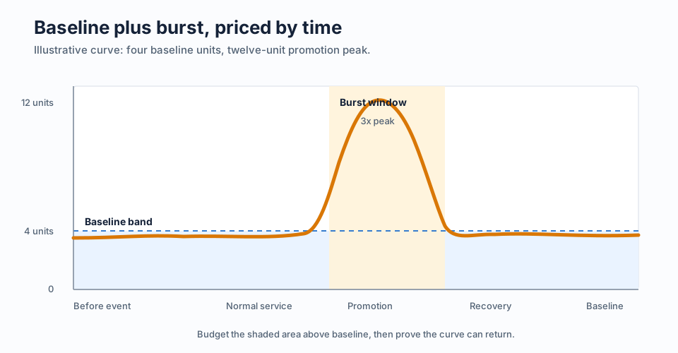
Provisioning to the maximum is attractive because it turns an uncertain event into a known fleet size. It also turns a short-lived requirement into a durable commitment. If a baseline needs four abstract capacity units and an annual promotion needs twelve, buying twelve for the whole year means carrying eight extra units for every non-promotion hour. A long commitment makes that decision harder to unwind when the traffic curve changes.
The first question is not "What is the peak?" It is "What must happen during the peak?" A producer path that must accept every event immediately has a different budget from an analytics consumer that can drain a backlog. Retrying connectors, catch-up reads, and log compaction also create different pressure than the initial write rate. Peak capacity only has meaning alongside a deadline, queueing tolerance, and recovery objective.
Write those service objectives down before comparing instances or autoscaling policies:
- Accept: the maximum producer rate the platform must acknowledge without throttling.
- Drain: the backlog or replay rate that must be cleared after the burst.
- Retain: the data that must remain available, including the retention window and any compaction behavior.
- Recover: the capacity and time required after a broker, storage path, or availability zone failure.
Those requirements explain why a three-times throughput event does not automatically require three times the long-term broker fleet. It may require more serving compute for a short interval, a larger write buffer, more object-storage access, or a controlled producer quota. The budget should show which one is actually being purchased.
2Baseline and burst deserve different budgets
The baseline is the capacity that protects ordinary service. It includes steady producer and consumer work, routine retention, normal partition placement, and a reserve for expected failures. The burst is the incremental capacity required for a defined rate and duration. Keeping the rows separate makes the budget explainable when the event is canceled or the business schedule changes.
For an illustrative workload, assume four baseline capacity units, a twelve-unit peak, and four promotion windows per month, each lasting six hours. The incremental burst is eight units for 24 unit-hours in the month. If the same eight units are held all month, using a 720-hour budgeting month, the extra compute line becomes 5,760 unit-hours. The arithmetic is not a provider price claim. It is a way to expose the idle-capacity decision before a provider rate, reservation discount, or license model is applied.
The monthly model can stay provider-neutral:
Monthly budget =
  baseline compute hours x baseline unit rate
+ burst compute hours x burst unit rate
+ retained data x storage rate
+ billed network volume x network rate
+ object-storage requests and access charges
+ platform license and operations charges
The model needs more than average throughput. Record peak rate, burst duration, event count, partition distribution, consumer fan-out, retention, compression, and failure reserve. A short write burst may add little retained data, while a replay or catch-up window can add substantial reads after producers return to normal.
| Budget row | Illustrative input | What the row answers |
|---|---|---|
| Baseline compute | 4 units x 720 hours | What stays online between events? |
| Burst compute | 8 extra units x 24 hours | What is paid only for promotion windows? |
| Retained storage | Ingest bytes x retention, adjusted for compaction | How much data remains after the burst? |
| Network | Replication, consumer reads, and cross-zone paths | Which bytes are billed outside compute? |
| Access and operations | Requests, retrieval, monitoring, and support | What does the storage pattern add? |
The table keeps storage and network visible. A broker-hours-only budget can miss cross-zone replication, object-storage requests, or retrieval charges. Provider pricing changes by region, traffic direction, purchase option, and private-network path, so fill the rates from current provider pages.
3Three strategies: reserve, schedule, scale on demand
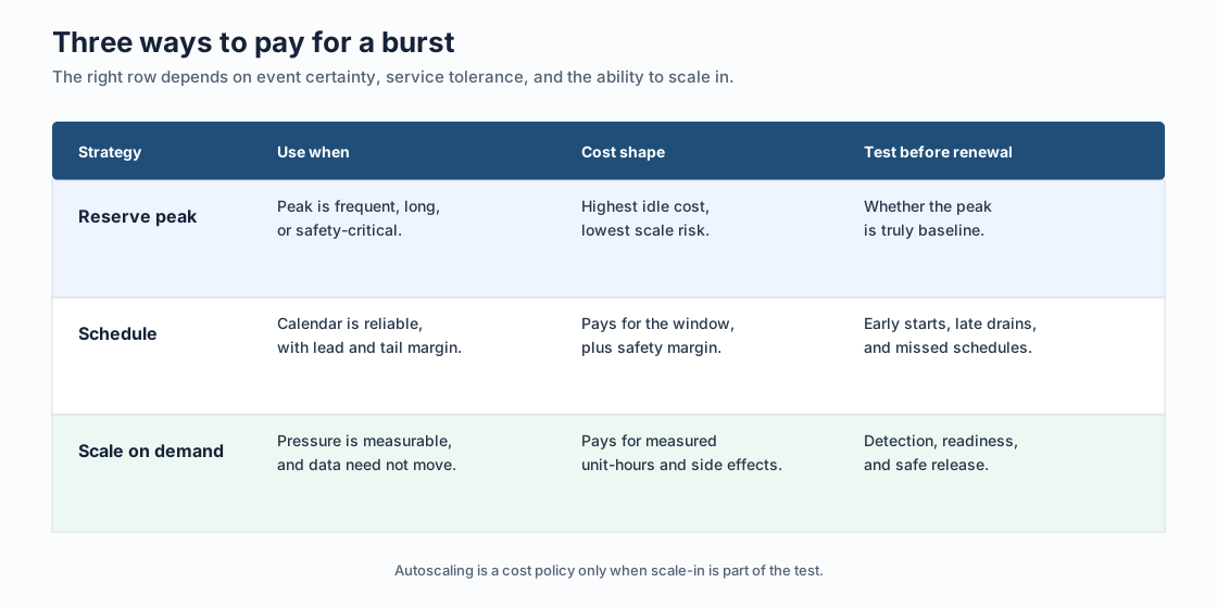
There are three useful ways to buy burst capacity. "Autoscaling" is not a budget strategy until its timing and scale-in behavior are measured.
Reserve the peak when the event is frequent, long, safety-critical, or too risky to change during execution. This works for a workload with a narrow latency objective and little tolerance for queueing. The trade-off is visible idle capacity. Put it in the budget as the price of immediate readiness rather than presenting it as ordinary baseline demand.
Schedule the peak when the calendar is reliable. A nightly batch, a known reporting window, or a planned promotion can trigger capacity ahead of time. Add a lead margin for provisioning and a tail margin for delayed consumers. Scheduled capacity is often easier to govern than a metric-driven policy, but it is still fixed capacity during the scheduled window. A calendar entry cannot detect an early campaign or a late replay.
Scale on demand when the platform can detect pressure, add serving capacity, and release it without moving durable data or breaking clients. The budget must include the scale-out signal, provisioning time, partition placement, warm-up, minimum capacity, and scale-in delay. It should also include what happens when the policy cannot act: producer quotas, backlog growth, or a temporary service-level exception.
The matrix is a decision aid, not a promise about any provider's implementation. "Fast" means fast enough for the stated service objective and must be tested in the target environment.
Spot capacity can fit the on-demand row for interruptible, stateless serving work, but it needs its own failure assumption. Test replacement capacity and interruption handling before tying durable storage, recovery guarantees, or a strict peak objective to a discount. A mixed fleet may reserve the minimum safe baseline and use interruptible capacity for work that can tolerate a restart or delayed drain.
4Why shrinking fast matters more than growing fast
Scale-out gets attention because it is visible during the incident. Scale-in determines whether the budget ever returns to baseline. If removing a broker requires copying partition replicas, draining local disks, waiting for reassignment, or coordinating a long maintenance window, the platform team may keep the extra capacity until the next event. The result is a successful peak response followed by permanent peak spending.
This is the storage boundary behind many Kafka autoscaling cost surprises. In a Shared Nothing architecture, brokers own local partition data and replicate it through leader and follower replicas. Adding or removing a broker can require partition reassignment while preserving replication health, min.insync.replicas, client routing, and recovery headroom. Apache Kafka's broker configuration reference and design documentation help map those controls to the workload.
Tiered Storage can change where older data lives, but it does not automatically make the broker fleet stateless. A deployment may still retain hot data locally, maintain replica placement, and pay for the network and request paths created by its access pattern. Treat retention and tiering as separate inputs to the budget, not as proof that scale-in is free.
The test should measure the full cycle: detect pressure, add capacity, become ready, serve or drain the burst, remove capacity, and return to baseline. Watch producer latency, consumer lag, partition movement, cache warm-up, storage requests, WAL behavior where applicable, and cross-zone traffic. If scale-in takes longer than the gap between events, the next budget period still carries peak capacity.
That requirement points to a different architecture property: durable data should not have to follow every compute change. The serving layer still needs capacity, routing, caches, and failure recovery, but the act of adding or removing a broker should be primarily a metadata and traffic operation rather than a full local-history migration.
5Deriving the storage and compute properties you need
The neutral requirement is specific. To avoid buying peak compute for the whole year, a platform needs all of the following:
- Kafka compatibility: existing producers, consumers, and operational tools should retain the Kafka protocol and semantics needed by the workload.
- Independent durable storage: retained bytes should remain available when serving compute changes, with a clear WAL and object-storage recovery boundary.
- A measured scale cycle: partition ownership, client connections, cache behavior, consumer lag, and failure recovery must be tested at the target burst shape.
- A complete cost meter: compute savings must be compared with WAL, object-storage requests, retrieval, network, monitoring, and license costs.
This is where a Kafka-compatible Shared Storage architecture becomes relevant. AutoMQ uses Separation of compute and storage: AutoMQ Brokers handle Kafka serving work while S3Stream writes durable stream data through WAL storage and S3 storage. Brokers can scale around serving capacity, ownership, metadata, and traffic rather than copying a full local log between nodes.
The storage details still matter. WAL (Write-Ahead Log) is a fixed-size, cyclic persistence buffer for durable writes and recovery before data reaches object storage. It is not the long-term retention layer. S3 storage holds durable stream data, while caching and compaction affect reads, requests, and cost. An AutoMQ WAL storage guide explains why the WAL type must be named in a cost test.
AutoMQ Open Source supports S3 WAL, while AutoMQ commercial editions support additional WAL storage choices depending on deployment and workload requirements. AutoMQ BYOC also keeps the control plane and data plane in the customer cloud account and VPC, which means the budget still needs to include customer-owned compute, storage, network, and marketplace or subscription charges. The deployment boundary changes who owns the line item; it does not remove the line item.
The claim is narrower than "elasticity is free." Shared Storage architecture can remove retained-data movement from broker scale changes. It does not remove partition hotspots, client limits, cache misses, object-storage access charges, WAL capacity, or slow consumers. Those remain in the test and budget.
6A budget model that survives the next promotion
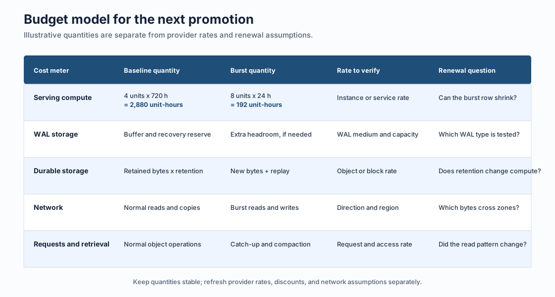
Use one worksheet for forecast, event review, and renewal planning. Keep rate assumptions separate from quantities so a region or provider change does not invalidate the workload model.
| Cost meter | Baseline quantity | Burst quantity | Rate to verify | Renewal question |
|---|---|---|---|---|
| Serving compute | Unit-hours outside events | Extra unit-hours during events | Instance, AKU, or service rate | Can the burst row shrink after the event? |
| WAL storage | Baseline buffer and recovery reserve | Extra buffer or throughput headroom | WAL medium and capacity rate | Is the WAL sized for the burst or the baseline? |
| Durable storage | Retained bytes and retention period | New bytes plus replay footprint | Object or block storage rate | Does longer retention change broker size? |
| Network | Normal reads and replication paths | Burst writes, reads, and cross-zone volume | Direction and region-specific rate | Which bytes leave the availability zone? |
| Requests and retrieval | Normal object operations | Catch-up, compaction, and replay requests | Request and access rates | Does the read pattern change after the event? |
For each promotion, record four timestamps: pressure detected, extra capacity ready, workload back to baseline, and capacity released. If the fourth timestamp is missing, the event has not finished from a FinOps perspective.
Renewal discussions should test the curve, not only the annual maximum. Ask whether the peak is becoming more frequent, whether the baseline has moved, whether retention has grown, and whether new consumer groups will multiply reads. A three-times event that repeats every week may belong in the baseline. A three-times event that lasts a few hours each year may belong in a burst budget. The right answer is a workload property, not a default setting.
Return to the Saturday promotion. If the team can state the baseline, price the eight extra units for the 24 illustrative burst hours, and prove that brokers can be released without moving durable history, it has a budget that matches the event. If it cannot prove release, the missing line is the cost of remaining at peak.
For teams evaluating a Kafka-compatible Shared Storage architecture against this worksheet, AutoMQ BYOC provides a customer-account path for a controlled workload test. Run the promotion curve, recovery case, and scale-in measurement together before changing a long-term compute commitment.
7References
- Apache Kafka design documentation
- Apache Kafka broker and topic configuration reference
- Apache Kafka quotas documentation
- Apache Kafka KIP-405: Kafka Tiered Storage
- AWS EC2 On-Demand pricing
- AWS EBS pricing
- AWS S3 pricing
- AutoMQ architecture overview
- AutoMQ Continuous Self-Balancing
8FAQ
8.1Should I buy Kafka capacity for the peak?
Buy for the peak when the event is frequent, long, safety-critical, or cannot tolerate a scale-out window. For a short, predictable event, separate baseline and burst capacity, then validate scheduled or on-demand capacity against the actual service objective.
8.2Does Kafka autoscaling reduce cost automatically?
No. It can reduce idle compute when it scales in safely and soon enough. It can also move cost into partition movement, replication traffic, storage requests, retrieval, or a prolonged oversize period. Measure the full scale cycle, including release.
8.3Is Tiered Storage the same as a Diskless architecture?
No. Tiered Storage can keep recent data on broker-local storage while offloading older data. A Diskless architecture makes durable stream storage independent from broker-local persistent disks. The retention, cache, WAL, and access model still need separate evaluation.
8.4What should I test before using spot capacity for a burst?
Test interruption handling, replacement capacity, client reconnects, partition ownership, consumer lag, and the recovery path. Use spot capacity for serving work whose disruption fits the service objective, and keep durable storage and recovery assumptions explicit.