
Table of Contents
Table of Contents
A Confluent Cloud cost calculator is only as good as the workload you put into it. That sounds obvious until renewal season arrives and the inputs come from last quarter's average bill, a few topic counts, and somebody's memory of peak traffic during a product launch. Kafka spend does not move like a flat subscription. It moves with bytes, partitions, retention windows, read fan-out, network paths, capacity headroom, and the boundary between what the managed service operates and what your cloud account still pays for.
Confluent's public pricing pages and billing documentation are useful starting points because they expose the categories a buyer has to reason about: ingress, egress, storage, cluster capacity, connectors, networking, support, and related platform services. The mistake is treating those categories as the model. They are the output columns. The input model belongs to the Kafka team, because only the platform owners know which workloads are steady, which spike, which replay, which retain data for audit, and which will be migrated or retired before the next contract ends.
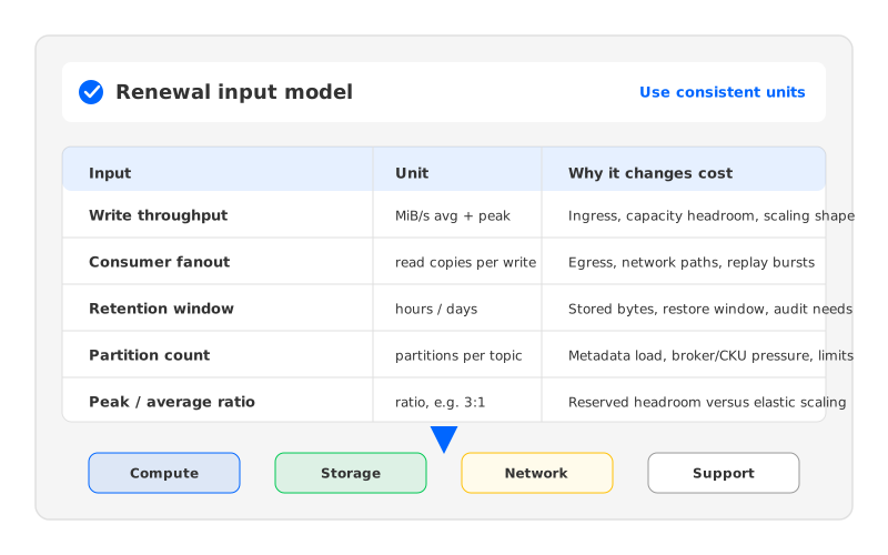
The practical goal before renewal is not to recreate Confluent's internal quote logic. It is to make the assumptions auditable enough that FinOps, procurement, SRE, and platform engineering can debate the same numbers. A good worksheet shows which workload characteristics create the bill and which architecture choices could change it.
1Why Kafka Cost Estimates Are Often Wrong
Many Kafka budgets begin with average throughput because it is easy to find. Average producer write rate, usually expressed in MiB/s, is necessary, but it hides workload shape. A topic writing 40 MiB/s all day behaves differently from a topic averaging 40 MiB/s because it idles overnight and bursts to 160 MiB/s during trading hours. Monthly volume may look similar, while capacity planning and throttling risk look very different.
The second source of error is read amplification. Kafka is a fan-out system by design. One byte written by a producer may be read by three stream processors, a search indexer, a warehouse ingest job, and a backfill consumer. If your worksheet only tracks producer ingress, it undercounts the consumer side of the platform. Confluent's billing model distinguishes dimensions such as ingress, egress, and storage; cloud providers also charge for network paths outside the managed service boundary. The same workload can therefore be economically quiet or noisy depending on where consumers run.
Retention is the third trap. Apache Kafka retention can be configured by time and size, and production teams often stretch retention after they discover replay, audit, or incident-recovery use cases. That changes the storage denominator from "today's traffic" to "traffic multiplied by retention hours or days."
| Estimation shortcut | What it misses | Better input |
|---|---|---|
| Average throughput only | Peak headroom, throttling risk, burst capacity | MiB/s average, MiB/s p95 or peak, peak/avg ratio |
| Producer ingress only | Consumer fan-out and replay reads | Consumer fanout as read copies per write |
| Topic count only | Metadata pressure and partition skew | Partition count by topic and environment |
| Current invoice only | Growth, retention changes, migration timing | Renewal-period forecast with scenarios |
| Service price only | Network, support, and operational boundary | End-to-end TCO worksheet |
Renewal is the point where the messy parts need names, units, owners, and ranges.
2The Workload Inputs You Need
Start with a single table that separates workload facts from vendor pricing. That discipline keeps the model portable. The same input row should be usable for Confluent Cloud, an Apache Kafka self-managed baseline, Amazon MSK, or a BYOC shared-storage alternative. If changing providers also changes the workload assumptions, you no longer have a comparison; you have two different stories.
At minimum, each application or workload group should include:
- Write throughput in MiB/s: record average, p95, and peak. Use MiB/s rather than MB/s so storage conversion stays consistent with infrastructure sizing.
- Consumer fanout: express this as read copies per write. A fanout of 4 means each written byte is read four times across steady consumers, not counting replays.
- Retention: record both retention hours and retention days. Hours matter for operational buffers; days matter for audit and replay economics.
- Partition count: track partition count by topic and by environment. Partitions affect metadata, balancing, limits, and capacity behavior.
- Peak/avg ratio: calculate peak MiB/s divided by average MiB/s. This number is often the difference between a calm renewal and an unpleasant capacity conversation.
Add message size distribution, compression ratio, environment count, DR requirements, private connectivity, and expected growth rate. They explain why a quote moves.
2.1Write Throughput and Peak Ratio
Throughput drives more than data volume. It influences whether a team needs serverless elasticity, dedicated capacity, reserved capacity, or a larger safety margin. Confluent documents different cluster types and capacity concepts, including Confluent Kafka Units for dedicated clusters and elastic Confluent Kafka Units for Freight clusters. Your contract may use private terms, but the workload still has to translate into capacity and usage.
Model write traffic with three numbers together: average MiB/s, peak MiB/s, and peak/avg ratio. A workload at 50 MiB/s average with a 2:1 peak ratio asks for different headroom than the same average with a 6:1 ratio.
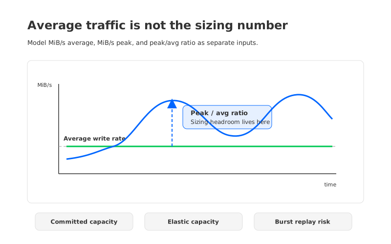
Do not hide spikes by converting everything into monthly TiB. Monthly volume helps storage reconciliation, but SREs size systems for the minute that hurts. FinOps needs both views.
2.2Read Fanout and Replay Behavior
Read fanout is easy to forget because it is not owned by one producer team. A platform topic can begin with one consumer and accumulate more over time as downstream teams discover it. That is good platform reuse, but it changes egress and capacity behavior.
Model steady reads separately from replay reads. Steady reads process near the head of the log. Replay reads happen during backfills, service bootstrap, DR tests, warehouse reloads, incident investigation, and migration validation.
A practical worksheet has two fanout columns:
- Steady fanout: the average number of active consumer copies per written byte during normal operation.
- Replay fanout: the expected number of historical rereads per month or quarter, with the largest replay window in hours or days.
If nobody knows replay behavior, write a range and assign an owner to measure it. A rough but owned range is better than a precise zero that everyone knows is fiction.
2.3Retention, Partitions, and Environments
Retention turns Kafka from a transport layer into a storage system. Kafka's documentation describes broker and topic-level settings for time-based and size-based retention. In a cost model, those settings become stored bytes: write MiB/s multiplied by seconds, adjusted by compression, replication or storage model, and retention duration.
Partitions create a different kind of cost pressure. They are not "bytes," but they influence metadata, leader placement, balancing, client behavior, and service limits. Track partitions by topic family and environment, because one heavily partitioned workload can drive scaling decisions out of proportion to its data volume.
Environment count matters because non-production Kafka is rarely free in practice. Development, staging, performance testing, DR, and migration environments can require capacity, retained data, connectors, network paths, or private endpoints.
3Networking and Support Inputs
Network cost is where managed-service estimates and cloud bills often drift apart. Confluent Cloud supports public endpoints and private networking options. Cloud providers then price data transfer, private connectivity, NAT, load balancing, and inter-region movement separately. AWS, for example, publishes separate pricing pages for EC2, EBS, S3, and VPC/networking services.
Before assigning dollars, draw the byte path. Producers may run in one VPC, consumers in another, analytics in a different account, and disaster recovery in a second region. A byte can be billed as ingress, egress, private connectivity traffic, cloud data transfer, or replicated storage. The model should show which side owns each bill.
Support and operations also need explicit treatment. Confluent Cloud provides managed operational value, and a fair renewal model should credit that value rather than pretending self-management is free. Topic governance, schema ownership, quota policy, client behavior, incidents, data contracts, and FinOps reporting remain customer work.
4How to Compare Confluent With BYOC Kafka Alternatives
An alternative evaluation should reuse the same workload table. If Confluent Cloud is modeled with average MiB/s, retention days, partition count, fanout, and peak/avg ratio, the alternative should accept those same inputs before adding architecture-specific fields. That keeps the comparison honest.
For a BYOC or self-managed Kafka option, the model usually expands into cloud primitives:
| Cost area | Inputs to capture | Typical source |
|---|---|---|
| Compute | Broker or compute-node type, count, CPU headroom, network bandwidth | Cloud provider EC2 or VM pricing |
| Block storage or WAL | Volume type, provisioned throughput, IOPS, durability boundary | EBS or equivalent storage pricing |
| Object storage | Stored bytes, request pattern, retention days, lifecycle policy | S3, GCS, Azure Blob, or equivalent pricing |
| Networking | Inter-AZ, inter-region, private endpoints, internet egress | Cloud networking pricing |
| Operations | Support, upgrades, observability, on-call ownership | Vendor contract and internal staffing model |
Include migration cost as a separate scenario rather than smearing it into the run rate. Inventory topics, ACLs, schemas, connectors, clients, quotas, retention policies, and consumer offsets. Budget for dual-run traffic, validation, rollback, and a period where both systems run.
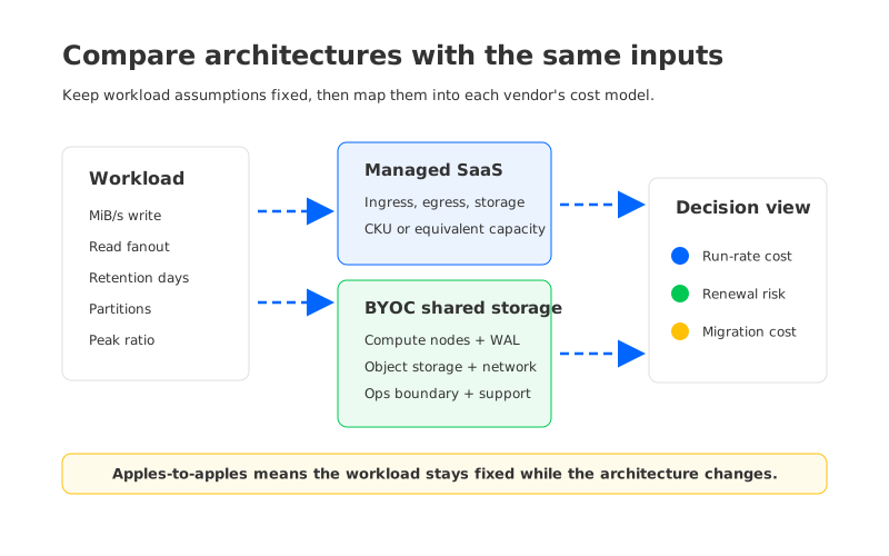
This is also the right place to separate technical fit from commercial fit. Some workloads may depend heavily on Confluent ecosystem services, governance workflows, or managed connectors. Others mainly need Kafka protocol compatibility, predictable cost, and control over the cloud account.
5AutoMQ Cost Modeling Considerations
AutoMQ belongs in the comparison as a Kafka-compatible, cloud-native streaming system that uses shared object storage as a primary part of the storage architecture. In cost modeling terms, the input table is remapped. Write throughput, consumer fanout, retention hours or days, partition count, and peak/avg ratio still matter. The question becomes how those inputs translate into compute nodes, object storage, WAL, network traffic, and the BYOC operational boundary.
Object storage is not merely a cold archive in this model. AutoMQ's architecture uses object storage for stream data while a WAL layer absorbs the low-latency write path, so the worksheet should separate object storage cost from WAL cost. That avoids a bad comparison where Confluent storage, traditional broker disks, and object storage are treated as interchangeable boxes.
For apples-to-apples evaluation, add these AutoMQ-specific rows to the same worksheet:
- Object storage: retained bytes by workload, request profile, retention days, and cloud-provider storage class assumptions.
- WAL: write MiB/s, peak MiB/s, durability scope, volume or file-system choice, and provisioned performance.
- Compute nodes: node type, count, CPU headroom, network bandwidth, and scaling policy.
- Network: producer and consumer locations, cross-AZ paths, private endpoints, replication, and replay traffic.
- BYOC boundary: which operations are automated by AutoMQ and which remain with the customer, including observability, change control, and support escalation.
This is not an argument that every Confluent workload should move. It is an argument that teams evaluating alternatives should compare architecture to architecture, not brand to brand. A managed SaaS platform bundles operational value into the service boundary. A BYOC shared-storage platform changes which cloud primitives appear on the bill and which operational controls stay in the customer's account.
The public AutoMQ pricing page is a useful companion to a Confluent renewal worksheet because it asks the same questions in a different architecture: write rate, retained data, reads, byte movement, and operational ownership.
6A Copyable Input Template for Renewal Reviews
The fastest way to improve a Confluent Cloud cost estimate is to make every assumption reviewable. Put this template in a spreadsheet, one row per workload or topic family, and keep units in the column names.
| Column | Unit | Owner |
|---|---|---|
| Workload name | text | Platform |
| Environment | prod / staging / dev / DR | Platform |
| Average write throughput | MiB/s | SRE |
| Peak write throughput | MiB/s | SRE |
| Peak/avg ratio | ratio | FinOps + SRE |
| Consumer fanout | read copies per write | Application owners |
| Replay window | hours or days | Application owners |
| Retention | hours and days | Data owner |
| Partition count | partitions | Platform |
| Compression ratio | ratio | SRE |
| Private networking | yes/no + path | Security + platform |
| Cross-region requirement | regions and direction | Architecture |
| Growth forecast | percent per quarter | Product + FinOps |
| Migration sensitivity | low / medium / high | Architecture |
After the first pass, group workloads into stable baseline, fast-growing, spiky, long-retention, high-fanout, and migration-candidate buckets. That grouping matters more than one grand total.
The renewal conversation gets healthier when the calculator is no longer a mysterious quote machine. It becomes a shared model of Kafka behavior. If the model says Confluent Cloud remains the right home for a workload, renew with clean assumptions. If it shows that retention, fanout, or cloud networking are driving the wrong cost curve, evaluate architecture changes before the contract makes those assumptions expensive to revisit.
7References
- Confluent Cloud Pricing
- Confluent Cloud billing overview
- Confluent Cloud networking documentation
- Apache Kafka documentation
- AWS EC2 On-Demand Pricing
- Amazon EBS Pricing
- Amazon S3 Pricing
- Amazon VPC Pricing
- AutoMQ Pricing
- AutoMQ Documentation
8FAQ
8.1What is the most important input for a Confluent Cloud cost calculator?
There is no single input. Average write throughput in MiB/s is necessary, but peak MiB/s, peak/avg ratio, consumer fanout, retention hours or days, partition count, and network path often explain the difference between a rough estimate and a renewal-ready model.
8.2Should FinOps use current Confluent invoices as the baseline?
Yes, but invoices should be evidence, not the whole model. Use current spend to reconcile the worksheet, then add workload-level inputs and renewal-period scenarios. That makes growth, retention changes, replay behavior, and migration timing visible before negotiation.
8.3How should teams model consumer fanout?
Use read copies per write. If one written byte is consumed by four steady downstream systems, the steady fanout is 4. Track replay fanout separately because backfills and migration validation can create short, expensive bursts that do not show up in average read behavior.
8.4How do retention days affect Kafka cost?
Retention multiplies stored data. A workload writing 20 MiB/s with 24 hours of retention and the same workload with 30 days of retention have very different storage profiles. Kafka retention settings are technical configuration, but in renewal planning they are financial assumptions.
8.5Where does AutoMQ fit in a Confluent renewal review?
AutoMQ fits in the alternative modeling step for teams that want Kafka compatibility with a BYOC shared-storage architecture. Model the same workload inputs, then map them to object storage, WAL, compute nodes, networking, and the operational boundary so the comparison remains apples-to-apples.