
Table of Contents
Table of Contents
An Apache Kafka dashboard can be green while a team is still paying for a growing backlog. Consumer lag may be climbing because a sink is slow, because one partition is hot, or because a storage path is waiting on I/O. At the same time, a network or retention change can increase the Google Cloud bill without moving the broker CPU graph. The useful dashboard is therefore not the one with the most charts. It is the one that connects a symptom to the path that produced it and to the decision an operator can take.
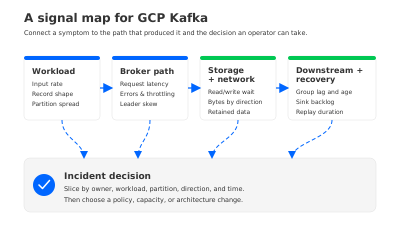
For Kafka on GCP, build that connection across four layers: workload demand, broker and partition behavior, storage and network, and downstream or recovery work. The Managed Service for Apache Kafka documentation describes the service surface; Cloud Monitoring's metric model explains how monitored resources and labels are represented. Your own Kafka exporters, connector metrics, billing export, and application telemetry fill the gaps between those surfaces.
1Start with a signal map, not an alert list
An alert says that something crossed a line. A signal map explains what the line means. Before setting thresholds, write down the path from a producer to a consumer or sink, then attach measurements to each boundary. This prevents the common mistake of treating “Kafka lag” as a single broker metric when it is actually the difference between a group's progress and the records available to it.
| Layer | Questions to answer | Useful signal families |
|---|---|---|
| Workload demand | Did the input rate or record shape change? | Produce bytes and records, request rate, record size, partition distribution |
| Broker and partition | Is Kafka accepting and serving the work? | Request latency percentiles, errors, throttling, leader skew, fetch and produce rates |
| Storage and network | Where do bytes wait or multiply? | Read/write latency, queue depth, bytes by direction, cross-zone path, retained data |
| Downstream and recovery | Can consumers, connectors, and recovery jobs keep up? | Group lag, record age, sink backlog, task state, replay rate, recovery duration |
The point of the map is ownership. A producer-rate increase belongs to the workload view. A hot partition belongs to partition placement or key distribution. A sink backlog belongs to the connector or destination team. When an alert names the owner as well as the symptom, the first response becomes a diagnosis instead of a dashboard tour.
2Consumer lag needs two clocks
Consumer lag is a progress signal: the consumer group has not reached the newest available offset. It is valuable because it shows whether a group is keeping pace, but it does not tell you why it is behind or how old the records are. A group reading large records slowly can have fewer lagging records than a group reading tiny records, while the first group still violates its freshness objective.
Track lag by group, topic, partition, and time window, then pair it with record age when the application can provide a timestamp. The useful alert is usually a sustained breach of the service objective, not a universal record count copied from another workload. Keep the threshold and evaluation window with the runbook so that an operator knows whether to inspect a hot partition, a paused consumer, a downstream dependency, or a temporary burst.
The two clocks are the consumer's position and the data's age. If lag rises while input rate is flat, inspect consumer processing, assignment changes, fetch behavior, and downstream calls. If lag rises only on one partition, inspect key distribution and leader placement. If lag rises during a replay, compare the replay rate with normal production and make the cost of those additional reads visible rather than labeling the event “broker overload.”
3Storage and network signals explain the bill
Cost analysis starts with bytes and boundaries. Retained bytes describe how much data the workload keeps; ingress and egress describe how much data crosses a service or network boundary; request and operation counts describe how often storage or APIs are called. A single “Kafka cost” number cannot tell you which policy or traffic path changed.
Use the same dimensions in operations and finance: project, region, cluster, topic or workload, client direction, and time window. Where the platform does not expose a topic-level cost dimension, estimate allocation from measured bytes and document the allocation rule. The estimate should be labeled as an allocation, not presented as a provider invoice.
Cost and health often move together, but the correlation is not proof. A replay can increase object reads and network bytes while reducing lag. A retention increase can grow storage spend without changing current throughput. A cross-zone consumer can raise network cost while broker request latency remains normal. Keep the billing export beside the technical dashboard and annotate changes such as retention policy, connector placement, replay, and scaling events.
4Connectors and recovery deserve their own panel
Connector dashboards are easy to under-specify because task status looks binary. A running task can still have a growing destination backlog, retrying records, or a freshness gap. Pair task state with source lag, destination write rate, retry counts, and the age of the oldest unprocessed record. If the connector has no native metric for a boundary you care about, emit that measurement from the connector wrapper or destination rather than guessing that “running” means “caught up.”
Recovery has a similar trap. A cluster can be available while a restore or replay is consuming storage and network capacity needed by live traffic. Record the start and end time of the operation, the amount of data read, the rate at which consumers catch up, and the point at which normal service objectives return. Those measurements turn a recovery exercise into evidence and make its cost explainable.
5A practical diagnosis sequence
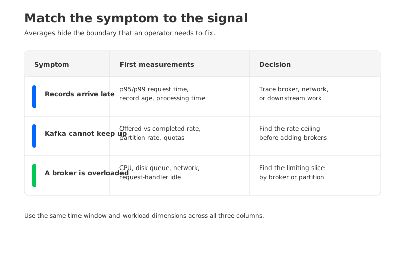
When lag, cost, or both move unexpectedly, preserve the time window before changing capacity. The following sequence keeps the first action tied to evidence:
- Name the symptom and boundary. Write down whether the problem is record age, request latency, throughput, spend, or recovery time, and identify the producer, group, connector, region, and topic involved.
- Compare offered and completed work. Check input rate against broker ingress, consumer delivery, and destination writes. A gap tells you which boundary to investigate next.
- Slice before averaging. Break the view down by partition, broker, client group, direction, and zone. Cluster averages can hide one hot partition or one expensive route.
- Correlate the cost event. Compare billing export or usage data with retention changes, replay, scaling, network placement, and connector activity in the same window.
- Test the recovery path. If the incident involves backlog or replay, measure the catch-up rate and the time to return to the freshness objective. Do not close the incident when the broker is merely healthy.
The sequence is deliberately conservative. It avoids changing a cluster before the team knows whether the limiting resource is the broker, the storage path, the network, or the application after fetch.
If the slice points to placement or local storage pressure, compare the evidence with a Kafka partition reassignment diagnosis. If retention or replay is the moving part, the Kafka storage and retention guide gives the storage-side context. Both links are useful only after the workload boundary has been identified.
6When storage architecture changes the dashboard
The signal map must follow the storage model. In a conventional Kafka deployment, broker-local storage, replication, partition movement, and disk queues are closely coupled to retained data. A full disk or a slow replica transfer can therefore explain both a lag incident and a scaling event.
That map changes when a Kafka-compatible platform separates broker compute from durable storage. AutoMQ is one such platform. Its Shared Storage architecture uses S3Stream and object storage for the durable data path while brokers handle Kafka protocol and compute responsibilities. Its Prometheus metrics documentation gives operators separate views of broker requests, cache behavior, WAL activity, and object-storage work.
That separation does not make every workload fast or every storage operation free. It changes the questions a dashboard can answer. A broker disk alert is no longer sufficient evidence for retained-data pressure; the operator should also inspect WAL behavior, cache effectiveness, object-storage access, and the network path serving cold reads. The same four-layer model still applies, but the storage layer now has more explicit boundaries.
7Build the runbook around decisions
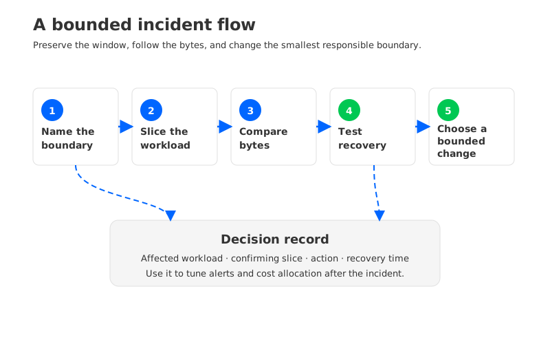
Every alert should link to a question and a next measurement. For lag, the question might be whether the group is processing slowly or receiving an uneven partition assignment. For cost, it might be whether bytes grew because of retention, replay, or network placement. For recovery, it might be whether the catch-up rate is improving or competing with live traffic.
Keep a small record with each incident: the affected workload, the first signal, the confirming slice, the action taken, and the time the objective recovered. Over time, that record exposes thresholds that are too sensitive, dimensions that are missing, and cost allocations that no longer match the architecture. It also gives platform and finance teams a shared vocabulary.
7.1Frequently asked questions
7.1.1What is the first metric to alert on for GCP Kafka?
There is no universal first metric. Start with the workload's freshness or throughput objective, then alert on the signal that measures a breach at the relevant boundary. Consumer lag is useful when paired with record age, input rate, and partition context.
7.1.2Should Kafka cost be compared with broker CPU?
CPU is a capacity signal, not a bill. Compare cost with retained bytes, traffic direction, request or operation volume, replay, and the cloud resources that host the data path. CPU can remain stable while storage or network usage changes.
7.1.3How do I avoid inventing provider metric names?
Treat the Google Cloud console and API output as the source for currently available managed-service metrics. Use documented resource types and labels, and keep exporter-derived Kafka metrics clearly separated from provider metrics. Recheck the service documentation before publishing a dashboard template.
The next time a GCP Kafka dashboard turns red, start with the two clocks: where the consumer is, and how old the data is. Then follow the bytes to the boundary that moved. If you want to inspect a Kafka-compatible shared-storage design and its observable layers, explore AutoMQ on GitHub and map the same runbook to your own workload before changing capacity.