
Table of Contents
Table of Contents
A Kafka capacity spreadsheet can look precise while describing a workload that never existed. The average ingress is correct, the peak number came from a dashboard, and the retention window came from a policy document. Then a campaign creates a short burst, a consumer group replays old data, and the cluster spends the next planning cycle carrying capacity for several different problems at once.
The failure is treating capacity as one number. A production plan needs ingress shape, peak duration, retained bytes, consumer work, and a comparison with what the system actually did. Kafka capacity planning is a measurement loop before it becomes a broker count.
1A Kafka capacity plan starts with four measured inputs
Start with the traffic that the platform must serve, then separate the reasons that traffic consumes resources. The four inputs below are related, but they answer different questions:
| Input | Measure from production | Planning question |
|---|---|---|
| Ingress | Bytes written over time, by Topic and Partition where possible | How much data must the platform accept? |
| Peak shape | Peak rate, duration, recurrence, and distribution across Partitions | How long must extra serving capacity remain ready? |
| Retention | Retention policy plus actual bytes remaining after cleanup or compaction | How much durable data must remain available? |
| Consumer parallelism | Consumer groups, active consumers, fetched bytes, lag, and replay windows | How much read and coordination work does the workload create? |
Ingress is the starting point, not the answer. A rate averaging 100 MB/s can be flat, bursty, or concentrated in hot Partitions, and those shapes need different serving capacity even with the same daily byte count.
Retention turns ingress into stored bytes after compression, cleanup, and storage overhead. Consumer groups add read work: two groups that read every Record can create roughly twice the read demand, while an idle group that replays later creates a different pattern. Keep those distinctions instead of collapsing them into “messages per second.”
2Measure traffic as a shape, not a single peak
Build a time series that shows what happened before, during, and after a pressure event. Collect producer and broker bytes, consumer fetch volume, lag, Partition distribution, and retention state for the same window. Kafka’s monitoring documentation and broker configuration reference provide the vocabulary; dashboards and labels depend on the deployment.
Use a time bucket that is short enough to preserve the burst that could affect queueing or an SLO. Hourly averages can erase a short promotion spike. A raw maximum can be worse: one bad scrape or a brief retry storm may turn into a permanent fleet-size assumption. Keep at least three views of the curve: the normal baseline, the sustained high-water period, and the brief maximum with its duration.
The same rule applies across the read path. Record which Consumer groups were active, how many consumers were assigned to each group, how many bytes each group fetched, and whether it was tailing recent data or catching up from an older Offset. Consumer parallelism is bounded by the number of Partitions assigned to a group, but a large consumer count by itself does not tell you how much data the brokers served. Fetched bytes and lag over time are more useful capacity inputs than a count of application processes.
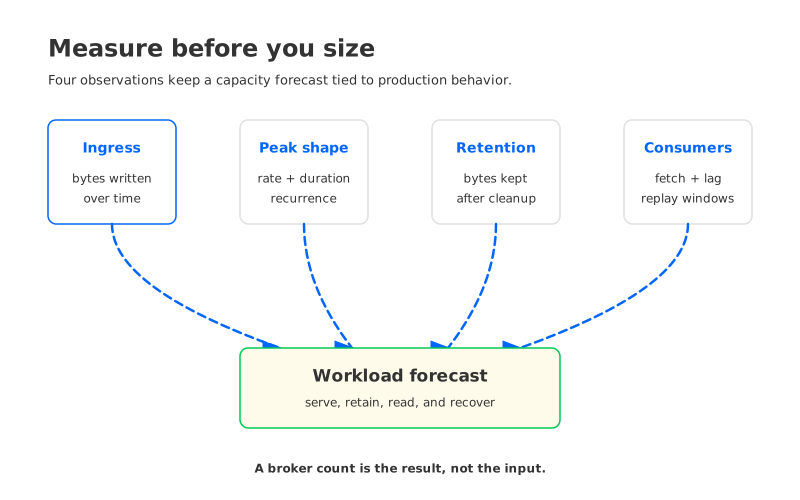
A useful sample includes the business cycle that creates the load and the recovery or replay activity that follows it. If a plan has only steady-state data, it has not measured peak shape; if it has only producer bytes, it has not measured the read path.
3Retention and consumers turn traffic into capacity
Retention is where a traffic forecast becomes a storage requirement. For a steady workload, a first estimate can multiply average ingress by the retention duration. That estimate becomes misleading when the curve is bursty, when compression changes by Topic, or when Log compaction removes older values. A better worksheet keeps time buckets and applies the retention rule to the bytes that actually remain available.
For an illustrative workload, assume 120 MB/s baseline ingress, a 10-minute peak of 300 MB/s, seven days of retention, and three Consumer groups. These are example inputs, not customer measurements. Seven days of uncompressed baseline ingress would be about 72.6 TB in decimal units. Compression, cleanup, compaction, and peak distribution can move the retained result.
The consumer side needs the same discipline. A tailing group creates continuous reads, while a batch group that catches up can create high read demand after producers return to normal. A replay may warm caches, increase object-storage reads, or compete with tailing consumers. Keep these paths separate:
- Tailing reads: recent data consumed close to the production rate.
- Catch-up reads: historical data consumed faster than it was originally produced.
- Fan-out reads: multiple groups reading the same records for different services.
- Coordination work: connections, Partition assignments, commits, and rebalances that rise with group and consumer activity.
Do not multiply ingress by the number of consumers. Measure fetched bytes for each group and its replay intervals. The model should explain why a group adds work, rather than assume every consumer reads the full Topic.
4Recalibrate the forecast until it explains the system
A capacity model earns trust when each revision removes a known blind spot. Compare the forecast with the same measurements after a representative cycle, then change the assumption the evidence disproved.
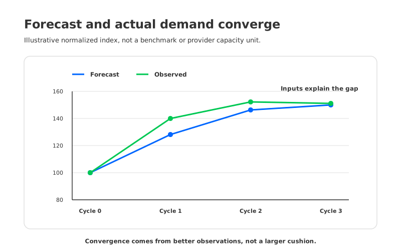
The following table is an illustrative convergence exercise. The demand index is normalized to the initial forecast, so it is a reasoning aid rather than a benchmark or a provider capacity unit.
| Planning cycle | Forecast assumption | Evidence from the next measurement window | Revised model |
|---|---|---|---|
| 0, baseline | 100 index points from steady ingress, seven-day retention, and three groups | No peak or replay window included | Add peak duration and read-path rows |
| 1, peak added | 128 points after adding the measured burst | Actual pressure reached 139 points during a short burst and a catch-up read | Split sustained peak from brief maximum; add catch-up bytes |
| 2, consumers added | 146 points after adding the fourth group | Observed demand reached 152 points, concentrated in two hot Partitions | Add Partition skew and group-specific fetch rates |
| 3, policy checked | 150 points with skew, replay, and retention included | Observed demand was 151 points across the same scenario | Keep the model and set the next recalibration trigger |
The numbers are intentionally normalized. What matters is the sequence: the first plan missed peak shape, the second missed consumer behavior, and the third missed Partition distribution. The model converged when its inputs described the workload that produced the pressure, not when the forecast was adjusted by a larger safety percentage.
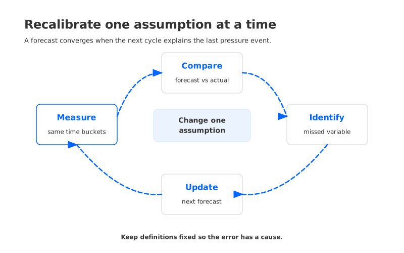
Use a fixed comparison sheet for each cycle. Keep metric definitions, time buckets, and units unchanged, then record the forecast, observed value, error, and changed assumption. Recalibrate after a new Consumer group, retention change, Partition expansion, compression change, or recurring peak appears. The result is a model with a known error budget and a reason to change, rather than a large unexplained cushion.
5Shared Storage changes the capacity vocabulary
In a traditional Shared Nothing architecture, the broker is both a serving process and the long-term owner of local Partition data. Capacity planning therefore ties together compute, local disk, replication, reassignment, recovery, and network traffic. Adding brokers can relieve serving pressure while creating data movement work. Adding disk can extend retention while leaving a hot Partition or a consumer replay bottleneck untouched.
A Shared Storage architecture separates those questions. Durable stream data has a shared storage owner, while brokers provide serving compute, routing, cache, and protocol handling. The planning unit is no longer “how many brokers hold the retained dataset?” It becomes a set of independently measured capacities:
| Capacity term | What to measure | Boundary that remains |
|---|---|---|
| Serving capacity | Ingress, egress, request rate, CPU, memory, and Partition skew | Hot Partitions and client limits can still dominate |
| Retention capacity | Bytes retained by time window and Topic policy | Object-storage capacity and access charges still apply |
| Write durability | WAL type, write rate, recovery reserve, and failure-domain behavior | WAL storage is part of the write path, not long-term retention |
| Read capacity | Tailing bytes, catch-up bytes, cache hit behavior, and replay concurrency | Cold reads can compete with live consumers |
| Recovery capacity | Broker replacement time, metadata recovery, storage access, and client recovery | A shared store does not remove protocol or network failure modes |
This vocabulary prevents a common category error. Object storage may remove broker-local disk as the durable placement constraint, but it does not make storage access free or make every read pattern equivalent. A capacity review still needs retention, object requests, WAL, cache, network, Partition count, and recovery scenarios. The architecture changes which row constrains the system; it does not remove the rows.
6Where AutoMQ fits in the measurement model
If the worksheet shows that retained data and broker lifecycle are coupled, the requirement is clear: keep Kafka semantics while giving durable data a storage boundary independent of serving compute. A Kafka-compatible Shared Storage architecture belongs in the comparison after the traffic model is explicit.
AutoMQ follows that model. Its S3Stream library replaces the native log-storage layer with a combination of WAL storage and S3 storage. AutoMQ Brokers handle Kafka traffic, while durable stream data is held in shared object storage. That separation lets a capacity exercise ask how much serving compute is needed for the measured ingress, egress, and Partition distribution without treating every broker change as a move of the full retained log.
WAL (Write-Ahead Log) still matters. It is the fixed-size persistence and recovery layer for writes that have not reached S3 storage, so the plan must name the selected WAL type and measure its write and recovery boundary. AutoMQ Open Source supports S3-compatible storage as its WAL option. AutoMQ commercial editions provide additional WAL storage choices for workloads and deployment models that need them. The choice changes the write-latency and failure-domain questions; it does not replace measurement.
AutoMQ’s continuous Self-Balancing documentation describes a controller that samples traffic and resource metrics to rebalance Partition assignments. That is useful only when the sampled metrics represent the workload you care about. A balancing mechanism can respond to the wrong window just as faithfully as it responds to the right one, so keep the same ingress, peak, consumer, and replay definitions in the evaluation.
AutoMQ maintains Kafka protocol compatibility, but compatibility is still a workload question. Validate the client versions, transactions, compaction, Connectors, security settings, and operational tooling your cluster uses. A Shared Storage architecture can change storage and reassignment behavior while leaving application-specific assumptions in place.
7A capacity worksheet you can run again
Keep one worksheet for ingress by time bucket, peak shape, retention, consumer read paths, recalibration history, and the architecture’s storage boundary. The same traffic can produce different operational work in broker-local and Shared Storage designs.
Before approving a capacity change, ask whether the decision can answer these questions:
- Which measured window sets the serving requirement, and how long does it last?
- Which Topic and Partition create the highest skew rather than the highest total volume?
- How many bytes remain under the actual retention and compaction policies?
- Which Consumer groups tail, catch up, or replay, and when do their read paths overlap?
- What changed between the last forecast and the next observation?
- If storage is shared, which WAL, cache, object-storage, network, and recovery limits now replace broker-local disk as the governing constraint?
Return to the spreadsheet that failed after the campaign. Repair it with a measured curve, a retention calculation, a consumer read map, and a recalibration record. To test that model against a Kafka-compatible Shared Storage deployment, start an AutoMQ BYOC evaluation with the same traffic windows, retention rules, consumer groups, and recovery objective.
8References
- Apache Kafka monitoring documentation
- Apache Kafka broker configuration reference
- Apache Kafka topic configuration reference
- Apache Kafka log compaction documentation
- Apache Kafka design documentation
- Apache Kafka KIP-405: Kafka Tiered Storage
- AutoMQ Shared Storage architecture
- AutoMQ S3Stream overview
- AutoMQ WAL storage
- AutoMQ compatibility with Apache Kafka
9FAQ
9.1What is the first metric to collect for Kafka capacity planning?
Start with bytes written over time, split by Topic and Partition when the telemetry allows it. Preserve the time buckets around ordinary traffic, sustained peaks, and brief bursts. Add consumer fetch bytes and lag in the same window before turning ingress into a cluster-size estimate.
9.2How should consumer groups affect a Kafka capacity model?
Model each group by the bytes it fetches, its tailing or catch-up behavior, and the Partitions assigned to it. Group count is a useful inventory field, but it is not a read-throughput multiplier by itself. A replaying group can create more pressure than a quiet group with the same number of consumers.
9.3How often should a Kafka capacity forecast be recalibrated?
Recalibrate after a complete workload cycle and after any change to retention, compression, Partition count, consumer groups, or peak behavior. The right interval follows the workload calendar. A fixed quarterly review can miss a weekly batch pattern, while an event-triggered review catches the changed input sooner.
9.4Does Shared Storage remove Kafka capacity planning?
No. It changes the units you plan. Durable retention moves away from broker-local disks, while serving compute, WAL, cache, object-storage access, network paths, Partition skew, and recovery still need measured limits.
9.5Is a Kafka capacity calculator enough?
A calculator is useful for checking arithmetic once the inputs are trustworthy. It cannot infer the shape of your peaks, the bytes fetched by each Consumer group, the retention result after compaction, or the recovery workload. Feed it measured distributions and keep a recalibration record beside the result.