
Table of Contents
Table of Contents
At an illustrative budget meeting, the platform lead brings an invoice showing $24,000 per month for a streaming estate that accepts 12 TB of logical records. Procurement has a vendor quote that implies $0.08 per GB. Finance says the cluster is expensive; the vendor says the quote is competitive; engineering says the two figures do not describe the same work. All three teams have done the arithmetic correctly. They have not agreed on what a gigabyte means.
That is the problem with most Kafka cost benchmarks. One number counts producer ingress, another counts compressed service bytes, and a third divides by retained storage or provisioned throughput. The result looks precise while the denominator moves underneath it.
The useful headline is dollars per streaming gigabyte. It is not a universal TCO metric and it does not replace reliability or migration analysis. It is a shared measuring stick: a declared numerator divided by a declared workload denominator, with the storage, network, and consumer boundaries written beside the result.
1Budget meetings need one number
The metric should answer a narrow question: how much did this platform spend to perform a defined amount of streaming work during a defined period? That question sounds obvious until a team tries to compare a self-managed Apache Kafka cluster, a managed service, and a Kafka-compatible shared-storage system. Their meters may cover broker-hours, partitions, throughput, retained bytes, requests, egress, or a bundled service unit.
Start with one workload class rather than averaging the whole estate. A compliance stream with long retention and an analytics stream with several replaying consumer groups create different economics even when their monthly ingress is identical. A single estate-wide number hides the reason the costs differ.
For a first comparison, use logical produced bytes as the headline denominator: the records accepted by the Producer before compression and before replication. That unit is closest to business demand and is usually available from application or Kafka metrics. It is only a starting point. Retained bytes and delivered bytes must be reported beside it when they drive the bill.
2Defining dollars per streamed gigabyte honestly
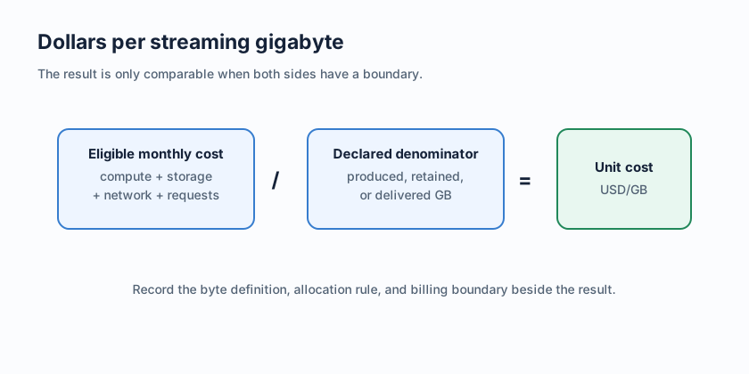
Write the metric as an equation before collecting prices:
dollars per streaming GB = eligible monthly cost / declared streaming GB
The numerator is the cost required to serve the selected workload during the measurement window. Depending on the platform, it can include compute, broker-attached storage, object storage, WAL storage, requests, retrieval, network transfer, private connectivity, support, and allocated shared-platform cost. Keep one-time migration or exit fees in a separate transition line.
The denominator needs a name, a unit system, and a boundary. Use decimal GB or binary GiB consistently; do not compare one vendor's GiB meter with another vendor's GB number without conversion. Then label which of these quantities the metric uses:
| Byte quantity | What it means | Where it can mislead |
|---|---|---|
| Logical produced GB | Application records accepted by the Kafka API before compression and replication | It does not show how many copies are stored or how many Consumers read the data |
| Compressed or wire GB | Bytes after compression on a request or network path | Compression settings can make two identical logical workloads look different |
| Retained GB-month | Bytes kept in durable storage over time | Retention, compaction, tiering, and replica policy change the quantity |
| Delivered GB | Bytes returned to Consumers, including fan-out and replay | One produced GB can become many delivered GB when several groups read it |
The safest headline is usually logical produced GB, with retained GB-month and delivered GB as companion metrics. For a replay-heavy analytics workload, delivered GB may be the more honest denominator for the read path. For a long-retention log, retained GB-month explains the storage bill that produced-GB alone would hide. The metric is not wrong when these numbers differ; the report is incomplete when it shows only one of them.
Avoid double counting. If a managed service bundles storage requests into a throughput charge, include the bundle once and document what it covers. If a cloud invoice separately shows object storage and request charges, keep both rows. If a network path is free under the provider's current pricing rules, record the zero as a verified assumption rather than silently deleting the path from the model.
3Collecting comparable samples across platforms
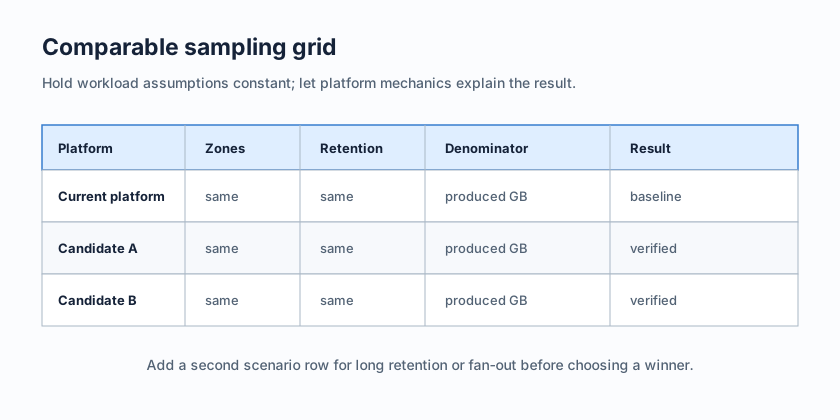
Comparability comes from holding the workload constant, not from asking every platform for the same marketing unit. Build a sample sheet with one row per platform and one column per assumption. The platform name is the least important column; zone placement, retention, compression, and consumer behavior usually explain more of the final number.
For each row, keep these inputs fixed:
- Workload shape: logical ingress, peak-to-average ratio, record-size distribution, compression, partitions, and batching.
- Durability target: replication factor or equivalent, acknowledgment behavior, failure domain, and recovery objective.
- Storage behavior: retention, compaction, hot and cold boundaries, storage class, and replay volume.
- Network shape: producer and Consumer placement, cross-AZ or cross-region paths, endpoints, connectors, and egress.
- Operating boundary: region, currency, billing period, support tier, deployment model, and shared-cost allocation.
Run the calculation across a normal period and a deliberately selected peak window. The normal period shows the cost of ordinary work; the peak window shows whether capacity is purchased for a short burst and then carried through the trough. A monthly average alone can reward over-provisioning that is invisible in the average. A peak-only result can punish a platform that scales with demand. Report both the workload shape and the unit cost.
| Sample row | Fixed inputs | Primary output |
|---|---|---|
| Long retention | Ingress, retention, compaction, failure domain, low replay | $/produced GB plus retained GB-month |
| Fan-out analytics | Ingress, Consumer groups, replay schedule, placement | $/delivered GB plus network cost |
| Bursty traffic | Ingress curve, peak window, scaling policy, headroom | $/produced GB plus peak compute cost |
4How the number gets gamed, and how to catch it
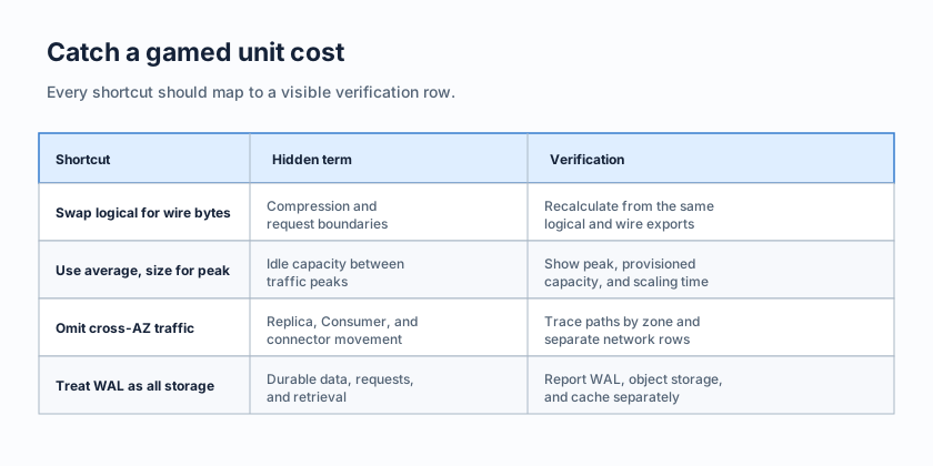
Most misleading unit costs are created by omission rather than an incorrect formula. A quote can be technically accurate and still be a poor comparison if it excludes the traffic, storage, or capacity needed to produce the quoted unit. Treat every headline number as a claim that needs a byte ledger.
| Common shortcut | What disappears | Check to run |
|---|---|---|
| Divide by logical ingress on one side and compressed bytes on the other | Compression and request-meter boundaries | Recalculate both platforms from the same logical and wire-byte exports |
| Use average throughput while sizing compute for peak | Idle capacity carried between peaks | Show average, p95 or declared peak, provisioned capacity, and scaling time |
| Exclude cross-AZ replication or consumer traffic | Network transfer and placement cost | Trace producer, Broker, replica, Consumer, connector, and storage paths by zone |
| Count storage price but omit requests or retrieval | Object storage access cost | Add request, retrieval, and replay rows from provider usage data |
| Stop the clock at the first write | Retention, compaction, and later replay | Add retained GB-month and delivered GB to the same workload row |
| Treat WAL as the whole storage layer | Durable object storage and WAL capacity | Separate WAL storage, S3 storage, requests, and cache behavior |
The last check matters for architectures that use a write-ahead log. WAL is a persistence and recovery boundary, not automatically the full retained dataset. A fixed-size WAL can support low-latency writes while older stream data lives elsewhere, but the model still needs the actual WAL allocation, durable storage, object requests, and read or retrieval behavior. The word "storage" is too broad for a defensible benchmark.
Ask for a reproducible calculation, not a better-sounding percentage. A reviewer should be able to change retention, compression, consumer count, or zone placement and see which rows move. If a vendor cannot disclose the meter boundary, mark that row unverified rather than filling the gap with an assumption favorable to the quote.
5Separate storage and network before choosing an architecture
After the byte ledger is complete, split the numerator into at least two architectural rows: durable storage and network movement. This separation is the point of the exercise. A platform can have a favorable storage rate and still lose the budget debate because replicas cross availability zones. Another can reduce broker disk usage while increasing object requests or cross-zone reads. The headline metric tells you which platform costs less for the selected work; the split explains why.
In a traditional Shared Nothing Kafka layout, each Broker owns local log data and replicas provide the durability and availability behavior. Retention ties durable bytes to broker capacity, and replication can create inter-zone traffic when the failure-domain policy places replicas in different zones. Apache Kafka settings such as replication and retention describe the behavior, but cloud billing decides which resulting paths are chargeable. Tiered Storage can move older segments to remote storage, yet it does not automatically erase active-log storage, replica movement, or Consumer locality from the model.
That gives the architecture review a concrete requirement: if storage and inter-zone replication are the dominant rows, look for a design that separates compute from durable storage and avoids copying the retained log between brokers for every capacity or placement change. The target is not a special denominator. The target is a different byte path that can be measured with the same denominator.
6Where AutoMQ fits the evaluation
If the sample shows that broker-local retained data and cross-AZ durability traffic are the drivers, a Shared Storage architecture becomes a relevant candidate. AutoMQ is a Kafka-compatible streaming platform built around that separation: its S3Stream storage layer uses shared object storage for durable stream data, while brokers focus on protocol handling, compute, and caching. The architecture documentation explains the storage boundary; the Kafka compatibility documentation defines the client-facing premise.
In this metric, the important change is not a lower denominator. It is the movement of cost rows. Durable data is measured in S3 storage and its requests, while the WAL path is measured separately. Stateless brokers can reduce the amount of retained data coupled to each compute node, and Self-Balancing can change how capacity is managed. Where the deployment topology supports it, AutoMQ documents zero cross-AZ traffic cost for the storage-driven durability path. Producer placement, Consumer reads, connectors, PrivateLink, cross-region replication, and egress still belong in the ledger.
The same discipline applies to AutoMQ BYOC. Cloud resources in the customer's account remain part of workload cost even if a separate platform fee appears on another invoice. Include compute, WAL, S3 storage, requests, network, support, and allocation rules in one numerator.
AutoMQ is therefore a scenario-dependent option, not the conclusion baked into the metric. It deserves a measured evaluation when long retention, broker-local storage, cross-AZ durability traffic, or storage-coupled scaling dominate. A short-lived, low-retention workload with little network exposure may not have enough of those costs for an architecture change to repay its migration effort.
7Put the metric in the monthly report
| Report field | Why it stays visible |
|---|---|
| $/logical produced GB | Common demand-normalized headline |
| Retained GB-month | Shows the cost of keeping history |
| $/delivered GB | Captures fan-out and replay work |
| Compute and storage split | Shows whether architecture or demand moved the result |
| Network transfer by boundary | Exposes cross-AZ, cross-region, endpoint, and egress paths |
| Peak-to-average ratio | Explains headroom and idle capacity |
| Assumption changes | Prevents a new codec, Consumer, or retention policy from looking like an unexplained trend |
Annotate the month when retention changes, a Consumer group is added, compaction behavior shifts, a new region is introduced, or the provider changes a billing definition. A falling $/produced GB can coexist with rising total spend because the business is streaming more data. A rising unit cost can be healthy if it reflects a deliberate retention or durability requirement. The report's job is to make that tradeoff legible.
Return to the budget meeting: the invoice is no longer divided by whichever gigabyte makes a quote look favorable. It is divided by a declared logical workload, with retained, delivered, storage, and network boundaries beside it. Take the next month's real usage exports and run the same worksheet against your current platform and an AutoMQ BYOC evaluation. Keep the producer bytes, retention, Consumer fan-out, zones, and recovery target fixed. The number will not end every debate, but it will make the remaining disagreement technical instead of semantic.
8References
- Apache Kafka documentation: Replication
- Apache Kafka documentation: Topic configurations
- Apache Kafka documentation: Quotas
- Apache Kafka KIP-405: Kafka Tiered Storage
- AWS Cost Explorer
- Amazon S3 pricing
- Amazon EBS pricing
- Amazon EC2 data transfer pricing
- AWS PrivateLink pricing
- AutoMQ Shared Storage architecture
- AutoMQ WAL storage
- AutoMQ zero cross-AZ traffic
9FAQ
9.1What should count in Kafka cost per GB?
Count the compute, storage, request, retrieval, network, support, and allocated platform costs required to serve the declared workload. State whether the denominator is logical produced GB, compressed wire GB, retained GB-month, or delivered GB. Keep one-time migration costs separate from steady-state unit cost.
9.2Why do Kafka cost-per-GB numbers disagree?
The teams are often pricing different bytes. Compression changes wire bytes, replication changes stored and transferred bytes, retention changes GB-month, and Consumer fan-out changes delivered bytes. Peak capacity, cross-AZ traffic, and bundled provider charges can change the numerator as well.
9.3Is logical produced GB always the best denominator?
It is a useful common headline because it follows application demand, but it is not sufficient for every workload. Long-retention streams need retained GB-month; replay-heavy or fan-out streams need delivered GB; bursty workloads need a visible compute and peak-capacity companion metric.
9.4Does Shared Storage remove every network cost?
No. It can change the durability path and may remove specific cross-AZ replication traffic under supported topology and configuration. Producer and Consumer placement, connectors, private connectivity, cross-region traffic, and egress still need to be measured.
9.5When should a team evaluate AutoMQ?
Evaluate it when the ledger shows that broker-local durable storage, cross-AZ durability traffic, retained-data growth, or storage-coupled scaling is a material cost driver, and when Kafka protocol compatibility is part of the requirement. Use the same workload, denominator, and migration checks for every candidate.