Redpanda Pricing Explained: How to Estimate Cloud Streaming Cost

People searching for Redpanda pricing are rarely asking only one question. The visible question is, "What will Redpanda cost?" The harder question is, "What will my cloud streaming platform cost once traffic, retention, replicas, network paths, managed fees, and operations are included?" Mixing those questions is how streaming budgets become surprising after a proof of concept looks successful.

Redpanda is a serious Kafka-compatible platform with multiple deployment models. Redpanda Cloud documentation describes Serverless, Dedicated, and BYOC-style options, and its billing documentation separates dimensions such as throughput, partitions, retention, requests, storage, and networking depending on the plan. Exact prices and allowances can change by date, region, and contract. That makes a static blog post a poor place to quote a durable unit price, but a good place to build the estimation model that keeps your comparison honest.

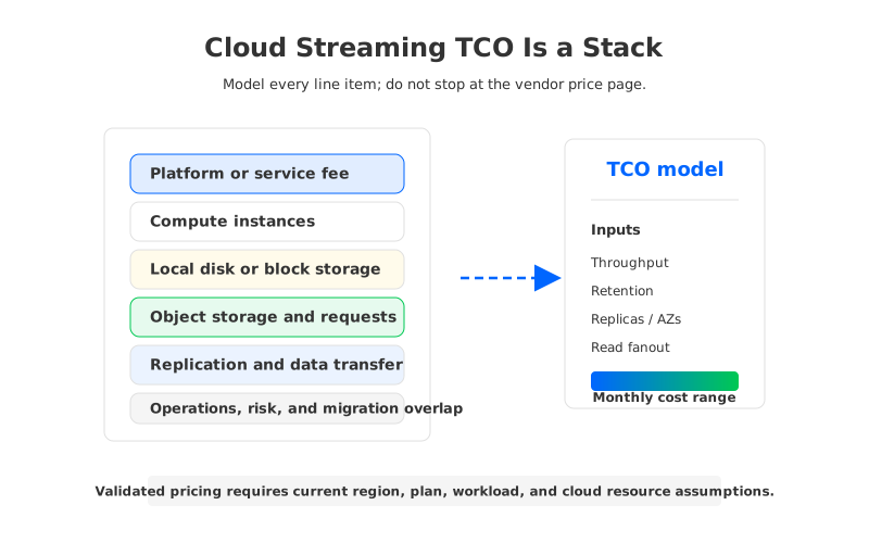
The right starting point is the full cost stack. A Kafka-compatible streaming system consumes compute, storage, network, and human attention. Managed service scope changes where those costs appear, but workload shape decides how large each part becomes.

What Redpanda Pricing Searches Often Miss

Redpanda pricing searches usually start with the vendor page because that is the most visible number. The vendor bill matters, but it is not enough for production TCO. Streaming infrastructure turns architecture choices into cloud line items: local disks become instance family decisions, replication becomes data transfer, retention becomes either hot storage or object storage, and peak traffic becomes headroom.

Redpanda's architecture is especially important to model because it is designed around high-performance local storage in many deployment patterns. That can be valuable for latency-sensitive workloads. It also means the cost model has to account for machines that own the log, storage attached to those machines, replicas needed for durability, and spare capacity for broker replacement or rolling operations. Tiered Storage can offload older data to object storage, but the hot local tier and reads that cross tiers still matter.

The useful question is which cost driver dominates your workload:

Hot-path performance. If tight produce latency is the constraint, the instance and storage choices that support that path may be warranted.
Long retention. If retained bytes grow faster than active throughput, storage architecture and tiering behavior may dominate the bill.
Read fanout and replay. If many consumers reread the same data or run large backfills, network paths and cache efficiency matter as much as write throughput.
Elasticity. If traffic peaks are short-lived, holding capacity after the peak may matter more than average MiB/s.
Operational ownership. If the team runs the data plane, staff time, incident load, upgrades, observability, and migration overlap belong in the model.

This is why Redpanda Cloud and self-managed Redpanda estimates need separate assumptions. The product may be the same family, but the bill lands in different places.

Redpanda Cloud vs Self-Managed Redpanda Cost Components

Redpanda Cloud pricing should be read through the service shape. Serverless emphasizes consumption-style billing. Dedicated is closer to provisioned cluster capacity and cloud resource shape. In BYOC, the platform may be managed by the vendor while underlying compute, storage, and network resources live in the customer's cloud account. For exact packaging, use Redpanda's current billing documentation and pricing estimator when you build the business case.

Self-managed Redpanda is different because the vendor subscription, if any, is only one input. The platform team owns more of the cloud architecture and operations. The upside is control. The cost is that every deployment choice must be modeled explicitly: instance type, local NVMe or block storage, availability-zone placement, replication factor, object storage for tiering, load balancers, monitoring, logging, backups, and labor.

Cost area	Redpanda Cloud estimate	Self-managed or BYOC estimate
Service fee	Current Redpanda plan, metering dimensions, committed spend, and support terms	License or support terms if applicable
Compute	Included, abstracted, or mapped to cluster capacity depending on plan	VM or Kubernetes node cost, CPU, memory, network, and overprovisioning
Storage	Retention and storage dimensions from official billing docs	Local disk or block storage, tiered object storage, snapshots, and spare capacity
Network	Ingress, egress, inter-zone traffic, private networking, and consumer location	Replication traffic, client traffic, object storage traffic, NAT or private endpoint cost
Operations	Partly included in managed service scope	SRE time, upgrades, balancing, incident response, observability, and migrations

The table is not a price list. A price list gets stale; a cost map stays useful. The most defensible estimate links each row to a dated source: Redpanda billing docs, cloud provider pricing pages, and your own telemetry.

The Workload Inputs That Drive Streaming TCO

A streaming TCO model should begin with workload telemetry, not node count. Node count is an output of the model. Start with how the workload behaves, then decide what Redpanda plan, instance shape, storage tier, or alternative architecture maps to it.

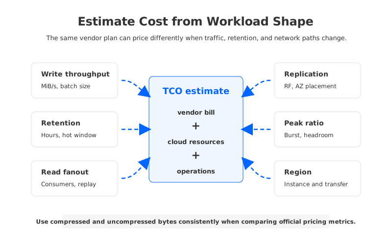
The base inputs are sustained write throughput, peak write throughput, retained data, read fanout, replay frequency, partition count, replication factor, availability-zone strategy, and cloud region. The tricky part is consistent units. Redpanda, Kafka, cloud storage, and network services may meter bytes in different forms; some dimensions may be logical or uncompressed while storage bills physical bytes after compression. Document the assumption rather than burying it in a formula cell.

Write Throughput and Replication

Write throughput is the first multiplier because it affects compute, storage growth, replication traffic, and request volume. A daily ingest estimate starts with write MiB/s × 86,400 seconds. Convert that to GiB or TiB, then apply the physical storage multiplier that matches the architecture. In a local-replicated Kafka-style model, usable retained data and physical stored data differ because replicas consume capacity. Apache Kafka's design documentation describes replication as the mechanism that keeps partition logs available across brokers; the cost model pays for those copies somewhere.

Replication also creates network questions. If replicas are spread across availability zones, durability improves, but cloud data transfer may enter the bill depending on provider rules and traffic direction. If consumers read across zones or regions, read traffic can become material even when the write path looks affordable. Durability, locality, and cost are one design decision.

Retention and Storage Tier

Retention is the quiet budget killer because it grows even when throughput feels stable. A workload writing a steady volume every day turns a seven-day retention policy into a storage multiple; a thirty-day policy multiplies it again. Local-storage systems need hot capacity for retained segments, compaction behavior, cushion, and broker replacement scenarios. If Tiered Storage is enabled, older data can move to object storage, but the hot tier still needs to serve current reads and writes.

For Redpanda, use official Tiered Storage documentation to understand what data can be offloaded and which reads may touch object storage. For cloud infrastructure, use the current object storage pricing page for capacity, request, retrieval, and data transfer terms. Avoid using a single "storage per GiB" cell unless the workload never performs large replays, creates many small objects, or crosses network boundaries. Streaming retention is not only bytes at rest; it is bytes being found, fetched, cached, and served later.

Read Fanout and Network Egress

Read fanout is often underestimated because many cost models focus on ingestion. A topic with one producer and ten independent consumer applications can generate much more read traffic than write traffic. Add replay jobs, backfills, late consumers, stream processors, and cross-region analytics, and the network model can become the difference between a plausible budget and a painful one.

Model read fanout as a first-class input. Steady consumers read near the tail and may benefit from cache locality. Replay consumers read older data, which may involve local disk, tiered object storage, or remote fetch paths. Cross-zone and external consumers can turn a normal fetch pattern into a data transfer or egress line item.

Managed service boundaries matter here. A vendor plan may include some traffic dimensions while the cloud account still sees private networking, endpoint, NAT, or inter-region charges. Read the billing docs and the cloud bill together.

How Shared-Storage Kafka Can Change the Cost Curve

At some point the cost question becomes architectural. If retained data is bound to broker-local disks, storage and compute scale together. If the workload needs more retained bytes, the cluster may need more or larger brokers even when CPU is not the bottleneck. If traffic drops after a peak, the team must consider where partition data lives and how much movement or rebalancing is required.

Shared-storage Kafka changes that premise. Durable data is placed in shared object storage or cloud storage, while brokers become more stateless and focus on protocol handling, scheduling, caching, and reads. A write-ahead log layer can absorb the low-latency write path before data is compacted or uploaded into object storage. The system still has costs, but the inputs change: compute, WAL storage, object storage capacity, object requests, cache hit rate, and network locality replace some local-disk and replica-placement pressure.

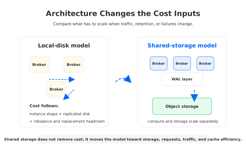
AutoMQ belongs in the discussion as a Kafka-compatible shared-storage system rather than as a generic "another vendor" line item. AutoMQ keeps the Kafka protocol and ecosystem expectations, but separates compute from storage with stateless brokers, WAL storage, and S3-compatible object storage as the durable layer. For TCO modeling, that changes the question from "How many brokers and disks do I need to hold the log?" to "How much compute do I need for active traffic, and how much shared storage do I need for retained data?"

That does not make every workload lower-cost by default. A low-latency workload with a small hot data set may value local-storage performance enough to support the Redpanda cost profile. A retention-heavy or elastic workload may benefit from a model where retained data growth does not force the same broker fleet growth. The honest comparison is workload-specific: use the same ingest, retention, read fanout, AZ placement, and failure assumptions across Redpanda and AutoMQ, then compare where the bill lands.

A Practical Estimation Checklist

The best Redpanda cost estimate is boring in the right way. It lists assumptions, links every price input to an official source, and shows the workload math in units the platform team can verify from telemetry. A range with clear assumptions is more useful than a precise number built on a guessed read fanout.

Use this checklist before presenting a Redpanda pricing estimate:

Record the plan and date. Capture whether the estimate uses Redpanda Serverless, Dedicated, BYOC, or self-managed deployment, and record the date you checked the official billing or pricing page.
Normalize workload units. Convert write throughput, retained bytes, and read traffic into consistent MiB/GiB/TiB units, and state whether bytes are compressed, uncompressed, or logical.
Separate vendor and cloud bills. Show Redpanda service fees separately from cloud compute, storage, object storage, data transfer, load balancing, logging, and monitoring.
Apply replication and headroom explicitly. Do not hide replication factor, availability-zone layout, failover capacity, or burst headroom inside an unexplained node count.
Model retention tiers. Distinguish hot local data, tiered object storage, long-term retained data, and replay behavior.
Include migration overlap. During migration, source and target clusters may both run, replication tools may add traffic, and teams may temporarily overprovision for rollback safety.
Run sensitivity analysis. Change peak ratio, read fanout, retention days, and cloud region. If a small assumption change breaks the budget, the architecture needs more scrutiny.

The last step is especially important for procurement. A streaming platform that looks attractive at average traffic may behave differently at peak traffic, after retention grows, or when another analytics team adds replay-heavy consumers. Cost modeling should expose those breakpoints before the contract is signed.

If your estimate shows that retained data, burst headroom, or broker replacement dominates the budget, compare Redpanda with a shared-storage Kafka design using the same workload telemetry. The next useful step is a workload-based assessment, not a generic platform demo. Talk to the AutoMQ team with the assumptions you want to test.

References

FAQ

How much does Redpanda cost?

Redpanda cost depends on the deployment model, current plan packaging, region, workload, retention, traffic, and cloud infrastructure. Use Redpanda's official pricing and billing pages for current service dimensions, then add cloud compute, storage, networking, and operations for a full TCO estimate.

Is Redpanda Cloud pricing the same as self-managed Redpanda cost?

No. Redpanda Cloud may include managed service scope and plan-specific metering, while self-managed Redpanda exposes more of the cloud infrastructure and labor cost directly. BYOC models often sit between those two: the vendor may manage parts of the platform, but the customer cloud account still carries the data-plane resources.

What is the biggest driver of Redpanda TCO?

It depends on workload shape. Low-latency workloads may be driven by compute and local storage choices. Retention-heavy workloads may be driven by storage and tiering. Read-heavy workloads may be driven by network paths, cache locality, and egress. The safest estimate treats all of these as variables rather than assuming one universal driver.

Does Tiered Storage make Redpanda cost close to object-storage-native Kafka?

Tiered Storage can reduce pressure on local disks by moving older data to object storage, but it is not the same cost model as a shared-storage architecture where object storage is the primary durable layer and brokers are more stateless. Both designs should be modeled with the same workload inputs.

When should AutoMQ be included in a Redpanda pricing evaluation?

Include AutoMQ when Kafka compatibility matters and the cost concern is tied to retention growth, elastic traffic, broker-local storage, or operational work around scaling and reassignment. AutoMQ's shared-storage architecture changes the TCO inputs by separating compute from durable storage, which can be relevant for BYOC and cloud-native streaming budgets.

Should I use a Redpanda cost calculator?

Use the official estimator or sales-provided calculator when available, but do not stop there. A calculator is only as good as its inputs. Validate write throughput, retention, read fanout, replication factor, cloud region, and migration overlap against production telemetry before using the output for a budget decision.