
Table of Contents
Table of Contents
Your Kafka budget review has six lines: broker instances, attached block storage, replication traffic, client traffic, retained data, and recovery or retrieval. The cluster accepts an illustrative 2 TB of logical records per day, keeps 14 days of history, uses a replication factor of 3 across three Availability Zones (AZs), and carries a peak several times its quiet-period load. The invoice does not identify the byte path, so the team argues about instance types.
That argument starts in the wrong place. Before changing the architecture, map every line to the work that creates it. In a broker-local Apache Kafka deployment, compute and durable storage are purchased together even when the workload needs one more than the other. Replication adds another byte path, and retention turns yesterday's traffic into today's capacity requirement. The useful question is not whether shared storage has a lower list price. It is which meters move when brokers no longer own the retained log.
1Start with the meters, not the architecture diagram
Write the budget as a ledger before comparing platforms. Use the same logical ingress, retention window, Consumer fan-out, durability target, AZ layout, compression policy, and recovery objective on both sides. Then separate the meters that are often hidden inside a single managed-service or node quote.
| Meter | What creates it | What to keep fixed in a comparison |
|---|---|---|
| Compute | Request processing, connections, Partition leadership, scheduling, and cache work | Peak load, partition count, connection count, and scaling policy |
| Storage | Durable bytes, WAL (Write-Ahead Log) capacity, local cache, or object storage | Retention, compression, compaction, and storage class |
| Replication | Copies made to satisfy the replication factor or durability policy | Failure domain, acknowledgment behavior, and replica policy |
| Network | Producer, Consumer, replica, connector, endpoint, and cross-region paths | Client placement, AZ topology, and egress destinations |
| Retention | Bytes kept over time, including compaction and segment cleanup behavior | Retention duration, retention.ms, retention.bytes, and cleanup policy |
| Retrieval | Reads of historical data, object GETs, prefetch, and replay | Consumer groups, replay frequency, catch-up window, and read locality |
This ledger prevents a common mistake: moving "storage" from a block-volume row to an object-storage row and calling the difference a saving. Storage may fall while request, retrieval, or network meters rise. Show that movement instead of hiding it in one total.
2The before bill couples capacity to retained bytes
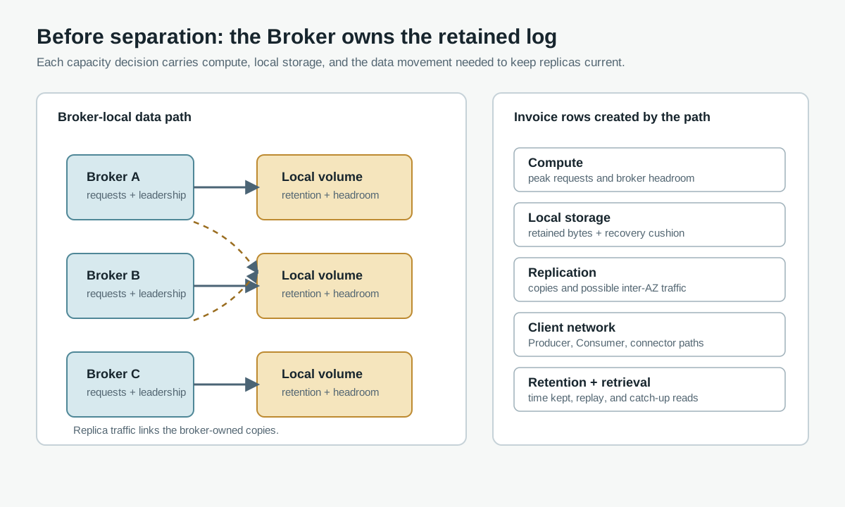
In the broker-local model, each Broker handles requests and owns local log segments. The volume must hold the retained data assigned to that Broker, plus headroom for recovery, segment movement, filesystem behavior, and a failure plan. Compute capacity is therefore sized with two curves in mind: the requests the Broker must serve and the bytes it must keep attached to itself.
That coupling matters during an ordinary capacity change. A traffic spike may require more request capacity, but adding a Broker also creates a data-placement problem. Partitions have to move, and moving them can mean reading and writing large amounts of retained data. A team may keep extra Brokers and disk capacity online because removing them later would trigger another rebalance. The budget line is not only the instance-hour; it is the capacity cushion that stays available because the storage cannot move independently.
The first bill has at least these rows:
- Broker compute: the fleet needed for peak request rate, connections, partitions, and operational headroom.
- Attached storage: block volumes sized for retention and recovery, including unused space reserved to avoid running full.
- Replication traffic: bytes copied from a leader to followers. With replicas spread across AZs, the path may become inter-zone traffic according to the cloud provider's rules.
- Client and export traffic: Producer writes, Consumer reads, connectors, monitoring exports, and cross-region destinations.
A replication factor of 3 does not mean every provider charges the same way for every copy, but it does mean the system performs more durable-write work than logical ingress suggests. For 2 TB/day of logical ingress, physical bytes depend on compression, batching, segment behavior, and replica placement. Do not multiply by 3 and call it an invoice. Use the multiplier to identify the path, then verify the provider meter and usage export.
3Retention and retrieval are different meters
Retention is a time-shaped cost. A record written once can occupy storage for one hour, 14 days, or longer, depending on policy. In a local-disk design, retention also determines how much capacity must remain attached to Brokers. In a shared-storage design, the durable bytes can be measured separately from the compute fleet, but they do not disappear.
Retrieval is the other half of the history decision. Tailing reads consume the newest data and may be served largely from cache or a write path. Catch-up Read pulls older data into the serving path, which can create object GETs, prefetch work, cache churn, and network movement. A compliance stream with long retention but rare replay may have a large storage row and a small retrieval row. An analytics stream with repeated replays can reverse that relationship.
Track at least these byte quantities in the worksheet:
- Logical produced bytes: records accepted by the Kafka API before compression and replication. This is the clearest demand denominator.
- Retained bytes over time: the storage footprint multiplied by the period it remains stored. This explains the retention meter.
- Delivered bytes: data returned to Consumers, including fan-out and replay. This explains read-side work.
- Physical and request bytes: compressed writes, replica transfers, object PUT or GET operations, and provider-specific retrieval units.
Do not force these quantities into one number. Report a primary denominator, then keep retained and delivered bytes beside it. Otherwise, producer ingress can look efficient while three Consumer groups reread the same history.
4What changes when compute and storage are separated
Separation changes the ownership boundary. Brokers still process Kafka requests, manage connections, lead partitions, schedule work, and serve data from cache. Durable stream data moves into shared storage, while a WAL provides a bounded write and recovery layer before data is uploaded or compacted into the long-term object store. The broker no longer needs to be the permanent home of every retained byte.
That changes the bill in four ways:
| After-side line | What may shrink or change | What still needs measurement |
|---|---|---|
| Broker compute | Capacity can follow request and cache demand more closely | Peak load, partition activity, connections, and cache hit behavior |
| Local persistent storage | May be removed or reduced to a cache or WAL role | WAL type, capacity, durability, and recovery behavior |
| Broker-to-broker replication | Durable record copies may no longer be the storage path | Metadata traffic, client traffic, and any remaining replication features |
| Shared object storage | Holds retained data independently of Broker count | Stored bytes, object requests, compaction, retrieval, and storage class |
The accounting does not become simpler; it becomes more explicit. Object storage can trade an attached-volume row for requests and retrieval. A WAL can lower write-path latency while retaining its own capacity and durability cost. A stateless broker can reduce the storage cushion attached to compute, while a read-heavy workload increases cache and retrieval work.
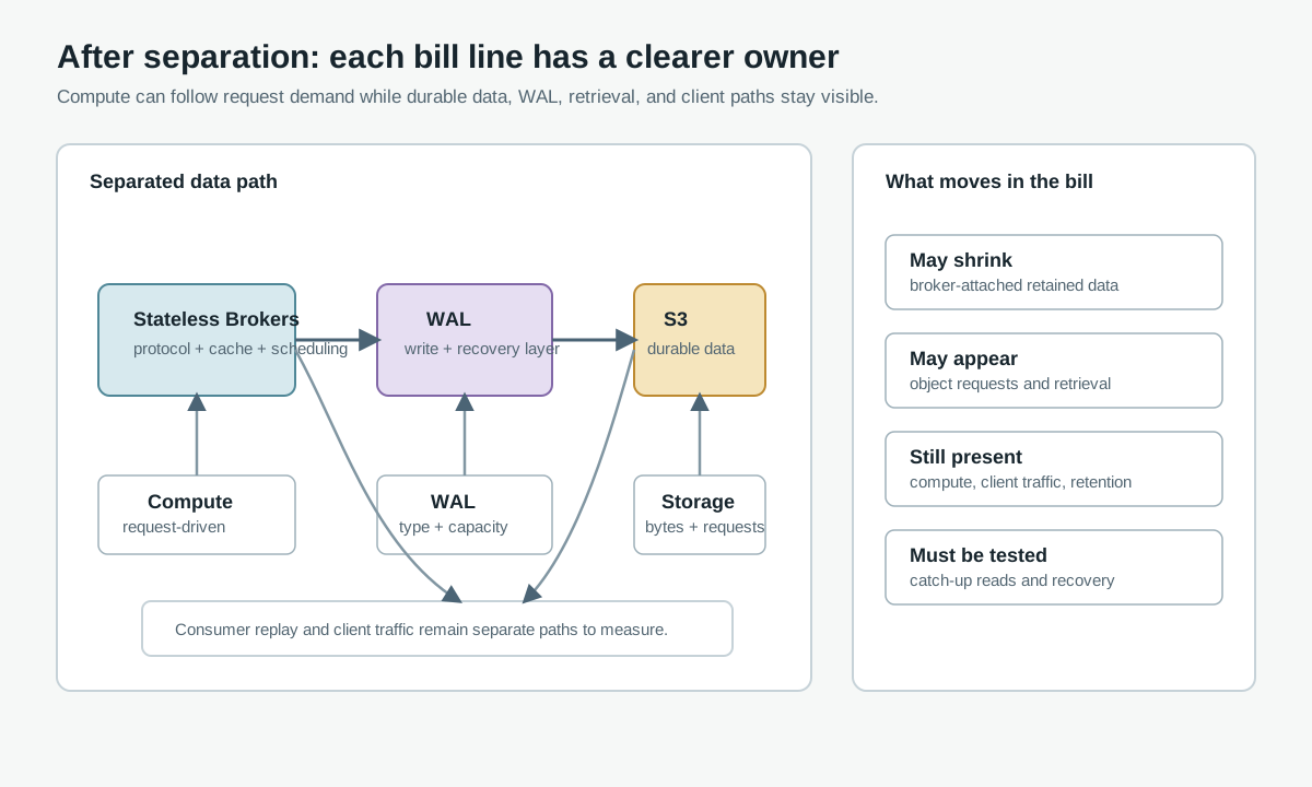
The benefit appears when the workload's dominant constraint is the old coupling. If Brokers are over-provisioned to carry retained data, or a scale event turns into a large partition-copy exercise, separation addresses the cause. If repeated cold reads dominate, the candidate must prove that retrieval and cache behavior meet the latency target and budget.
5Use a formula that exposes the trade-off
Do not begin with a provider price table. Begin with two totals whose rows have the same boundaries:
before = compute + local storage + replica traffic + client traffic
       + retrieval + operations

after  = compute + WAL + shared storage + object requests
       + retrieval + client traffic + operations

retention = an input that sizes local or shared storage, not a third storage charge

net change = after - before
This is a comparison model, not a promise. Keep one-time migration cost separate from steady-state economics. Add support, private connectivity, cross-region replication, and observability when they belong to the production boundary. If a provider bundles a meter, document what it covers instead of assigning the charge to a convenient row.
For the illustrative 2 TB/day workload, calculate three profiles instead of one blended average:
| Profile | Dominant pressure | Question the model must answer |
|---|---|---|
| Short retention, tail-heavy | Request processing and cache | Can compute follow the traffic without paying for unused retained capacity? |
| Long retention, infrequent replay | Durable storage and capacity coupling | Does moving history out of Brokers reduce the capacity cushion enough to offset shared-storage requests? |
| Replay-heavy analytics | Retrieval, cache churn, and network | Do object reads and prefetch add more cost than the local-disk design removed? |
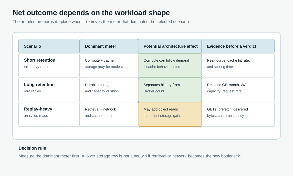
The same architecture can land differently for each profile. That is not an inconsistency. It is the reason to make retention and retrieval visible instead of quoting one average cost per GB.
6The required properties are clear before a product enters the discussion
The ledger points to a specific requirement: durable data needs a lifecycle independent of Broker count, and recovery must not turn every Broker change into a full retained-log copy. A candidate also needs a clear read path, an explicit WAL choice, Kafka protocol compatibility, and tests for client and Consumer behavior. Ask whether the WAL is S3 WAL, Regional EBS WAL, or NFS WAL, whether the storage path crosses AZ boundaries, and whether catch-up reads dominate requests.
7Where AutoMQ fits the line-by-line model
AutoMQ is a Kafka-compatible streaming platform that implements this class of design through its Shared Storage architecture. Its architecture documentation describes the boundary between Kafka request handling and the S3Stream storage layer. The relevance here is not a claim that every line gets smaller. It is that the lines map to different responsibilities.
With AutoMQ, durable stream data is stored through S3Stream and S3-compatible object storage, while WAL storage and data caching handle write and read behavior around that durable layer. AutoMQ Brokers are stateless with respect to persistent stream data, so scaling or replacing compute does not require treating each retained Partition as permanently attached to one node. The Shared Storage documentation is the place to verify the storage mechanics and deployment assumptions.
The bill still includes compute, WAL, object storage, requests, retrieval, client traffic, and the resources in the selected deployment model. Under a supported S3-based topology, the storage-driven durability path can avoid broker-to-broker cross-AZ replication traffic, but producer placement, Consumer reads, connectors, PrivateLink, cross-region traffic, and egress remain workload-specific rows. AutoMQ's zero cross-AZ traffic documentation describes the supported mechanism and its boundary.
AutoMQ is a candidate for a particular bill shape, not a conclusion inserted into the worksheet. Evaluate it when local retained data, cross-AZ durability traffic, or storage-coupled scaling is material and Kafka compatibility is required. A small, short-retention workload with little replay may not justify a migration.
8Turn the worksheet into a decision
Run the current and candidate designs through the same sequence:
- Export logical ingress, retained bytes, Consumer delivery, replay, and peak load for a representative period.
- Draw the producer, Broker, replica, storage, Consumer, connector, and egress paths by AZ and region.
- Label each path as compute, storage, replication, network, retention, or retrieval, then attach the provider meter or mark it unverified.
- Recalculate the three workload profiles after changing only the architecture-specific rows.
- Test recovery, scale-out, scale-in, and catch-up reads before treating the estimate as a production decision.
The result should show money and work. A lower steady-state total matters, but so does removing data-copy work from capacity changes. Keep retrieval behavior and operational effort beside the invoice result.
Return to the opening budget: 2 TB/day, 14 days of history, three AZs, and a peak that drives the fleet. The question is no longer "Which Broker instance has the lower cost?" It is "Which bytes require Brokers, which bytes require durable storage, and which paths are we paying to copy or retrieve?" Build that ledger with usage exports, then run a production-shaped AutoMQ BYOC evaluation with retention, replay, AZ placement, and recovery held constant.
9References
- Apache Kafka design documentation
- Apache Kafka replication documentation
- Apache Kafka topic configurations
- Apache Kafka KIP-405: Kafka Tiered Storage
- Amazon EBS pricing
- Amazon S3 pricing
- Amazon EC2 data transfer pricing
- AWS PrivateLink pricing
- AutoMQ architecture overview
10FAQ
10.1What does separating Kafka compute from storage change?
It changes which resource owns durable data. Brokers continue to handle Kafka requests, partition leadership, connections, and cache work, while shared storage holds retained stream data. The bill can then measure compute, WAL, durable storage, requests, network, retention, and retrieval as separate rows.
10.2Does disaggregated storage always lower Kafka cost?
No. The outcome depends on retention, Consumer fan-out, replay frequency, object requests, retrieval, network topology, WAL choice, and the capacity cushion in the existing cluster. A long-retention workload may have a different result from a replay-heavy workload even with the same logical ingress.
10.3What should a Kafka architecture cost comparison include?
Include compute, local or shared storage, WAL, replication, client network, cross-AZ and cross-region paths, object requests, retrieval, egress, support, operations, migration, and the same durability and recovery objectives. Keep the logical produced bytes, retained bytes, and delivered bytes visible so the denominator does not hide work.
10.4Is Shared Storage the same as Tiered Storage?
No. Tiered Storage typically moves older data to remote storage while a local log remains part of the serving design. A Shared Storage architecture makes shared durable storage the primary data layer and separates it from Broker compute. Evaluate the actual read, write, recovery, and retention paths instead of treating the terms as interchangeable.
10.5When should a team evaluate AutoMQ?
Evaluate it when the ledger shows that Broker-local retention, cross-AZ durability traffic, or storage-coupled scaling is a material constraint, and when Kafka protocol compatibility matters. Use the same workload profiles, cost boundaries, failure tests, and migration checks for AutoMQ and every other candidate.