
Table of Contents
Table of Contents
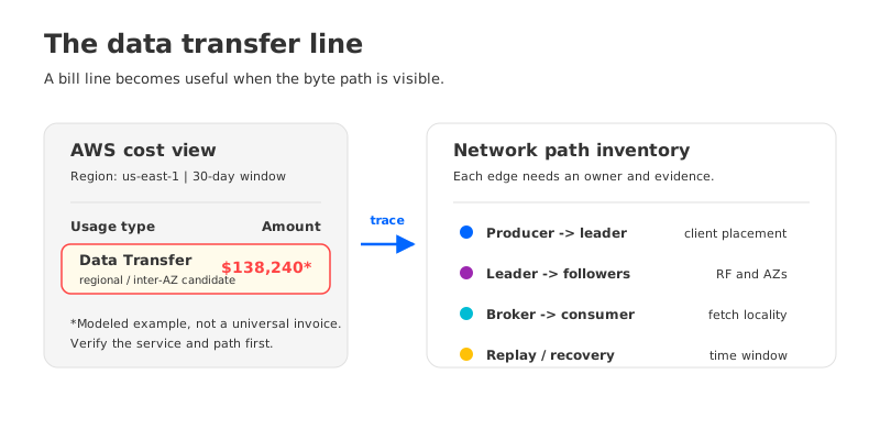
The line may read Data Transfer, Regional Data Transfer, or a similar usage type. It sits beside compute and storage, so a Kafka team can easily treat it as background AWS overhead. Then a traffic increase arrives, the broker count barely changes, and the line grows faster than the workload everyone thought they were paying for.
That is a billing problem before it is a Kafka problem. AWS prices data movement according to the path bytes take through the region. Kafka adds paths for leaders, replicas, consumers, replays, and recovery. A single logical record can therefore produce several physical transfers, some of which cross Availability Zones and some of which do not. The useful question is not "Why is Kafka charging me for ingress?" It is "Which Kafka path produced this metered transfer?"
The answer determines the remedy. A misplaced consumer can be fixed with scheduling or rack-aware reads. A necessary cross-AZ durability path may be a property of the storage architecture. The rest of this article separates those cases and gives you a bounded calculation before you change a cluster.
1The line you skim is a topology question
AWS does not need to know that a byte belongs to a Kafka record to meter it. It sees network interfaces, regions, Availability Zones, service boundaries, and directions. That is why the same Kafka workload can produce different data transfer costs after a placement change even when application throughput is unchanged.
Start by identifying the deployment boundary. A self-managed Kafka cluster on EC2, a Kubernetes cluster using EC2 nodes, and Amazon MSK do not expose exactly the same pricing treatment. AWS's EC2 On-Demand pricing says that data transferred in and out from specified EC2-related resources across Availability Zones in the same Region is charged at $0.01/GB in each direction. Amazon MSK's pricing page separately states that broker-to-broker replication is not charged as data transfer, while standard AWS transfer charges apply to data transferred in and out of MSK clusters.
Those statements are not contradictory. They describe different meters and service boundaries. Use the EC2 rate as an explicit assumption for an eligible self-managed path; do not apply it automatically to every byte inside MSK.
For an initial investigation, classify the traffic into paths rather than services:
| Path | What to ask | Useful evidence |
|---|---|---|
| Producer to leader | Is the client in the leader's AZ? | Client placement, broker placement, producer bytes |
| Leader to follower | Which replica hops cross AZs? | Replica assignment, broker interfaces, flow records |
| Broker to consumer | Are consumers reading locally? | Consumer placement, client.rack, fetch bytes |
| Replay or recovery | Did a job or failure change the read shape? | Job history, reassignment events, fetch rate |
| Export or connector | Is data leaving the cluster boundary? | Endpoint, NAT, PrivateLink, or destination metrics |
This classification prevents a common accounting error: attributing the whole Data Transfer line to replication because replication is the most visible Kafka mechanism. It may be the largest contributor, but consumer fan-out, a cross-zone producer fleet, or a recovery operation can be the event that moved the bill.
2Why replication creates a multiplier
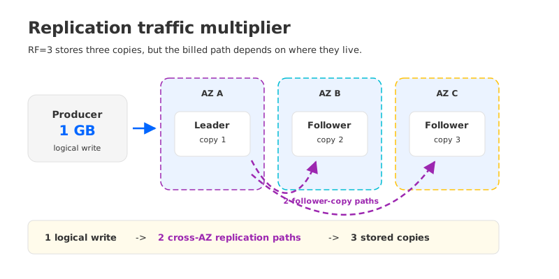
Kafka's durability model stores a partition on a leader and one or more followers. With a replication factor of three, one logical write has two follower copies to maintain. If the followers are in other AZs, the leader-to-follower movement is cross-AZ traffic. In a three-AZ layout, the placement is often intentional: each zone holds a replica so that a zone failure does not remove every copy.
That resilience choice changes the arithmetic. For each 1 GB written to a partition, the leader may send 2 GB to its followers. The producer-to-leader path can add another cross-AZ component when producers are spread across zones and partitions are not routed to a local broker. A consumer group can add still more movement if it fetches from a broker in another zone. Recovery and reassignment are bursts on the same graph, not exceptions that make the graph disappear.
The phrase "replication doubles the traffic" is therefore useful as a starting point, not as an invoice formula. It describes two follower-copy paths for RF=3. It does not include producer placement, consumer placement, compression, protocol overhead, retransmits, or whether the cloud service charges that path. Treat each term as a measurable coefficient.
The service qualification matters especially for managed Kafka. For Amazon MSK, AWS says broker replication is not separately charged. That does not make topology irrelevant: client traffic into and out of the cluster, cross-region movement, public internet egress, PrivateLink, and other connected services can still create billable transfer. A managed service may remove one line from the arithmetic without removing the physical paths from the architecture.
3A minimal model: 1 GB/s, three zones, one month
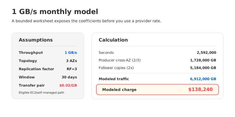
Use a deliberately narrow model to make the multiplier visible. The following example is for an eligible EC2/self-managed path with these assumptions:
- Logical producer throughput is 1 GB/s using decimal gigabytes.
- The cluster runs across three AZs with RF=3.
- Partitions and producers are evenly distributed, so two-thirds of producer traffic crosses from a producer to a remote leader.
- Both follower copies cross an AZ boundary, adding 2 GB of replication traffic for each 1 GB written.
- The month has 30 days, or 2,592,000 seconds.
- The applicable path is charged at $0.01/GB in each direction, represented as a $0.02/GB two-sided transfer pair.
- Consumer reads, replay, recovery, compression, and protocol overhead are excluded.
The worksheet is:
seconds in month             = 30 x 24 x 60 x 60 = 2,592,000
logical bytes written         = 1 GB/s x 2,592,000 s = 2,592,000 GB
producer cross-AZ traffic     = 2,592,000 GB x 2/3 = 1,728,000 GB
RF=3 replication traffic      = 2,592,000 GB x 2   = 5,184,000 GB
modeled cross-AZ traffic      = 6,912,000 GB
modeled transfer charge       = 6,912,000 GB x USD 0.02/GB = USD 138,240
The result is a scale illustration, not a promise that an AWS bill will contain exactly $138,240. It assumes every listed path is eligible for the rate and that the two sides of the inter-AZ path are both metered as described. It also excludes consumer traffic, which can be material when many readers are placed outside the brokers' zones. If one consumer group reads 1 GB/s across an AZ boundary for the same month, its additional two-sided candidate is another 2,592,000 GB, or $51,840 under the same assumptions.
The formula is more durable than the example:
candidate charge = P x (producer_cross_AZ + replication_cross_AZ + consumer_cross_AZ)
                   x seconds x applicable_rate
Define P carefully. Application payload, compressed producer bytes, and broker-observed bytes are not interchangeable. If compression reduces the wire volume, use the measurement that matches the billing path. If the provider bills only one side of a particular service boundary, use that service's rate instead of the two-sided pair. Keep the assumptions next to the result so Finance and platform engineering can reproduce it.
This model also explains why retention alone cannot explain a sudden Data Transfer increase. Retention changes how much data remains available; it does not by itself create a new network path. A new consumer group, a zone-skewed deployment, a partition reassignment, or a replay job can change the transfer coefficient while logical ingress stays flat.
4Verifying the traffic with Cost Explorer and Flow Logs
The investigation should end with a path that another engineer can reproduce. Use a matching time window and move from the bill to the network evidence, then back to Kafka metrics.
- Start in Cost Explorer. Filter the account and Region, then group the period by service and usage type. Preserve the exact usage type, operation, and linked account that contain the increase. AWS's Cost Explorer documentation describes the tool's filtering and grouping model. A generic "data transfer" total is not enough for attribution.
- Map interfaces and zones. Use VPC Flow Logs or an equivalent network record to compare source and destination ENIs, AZs, bytes, and timestamps. Flow Logs can show that two interfaces exchanged bytes across zones; they cannot tell you which topic or partition produced those bytes. Keep that limitation in the report.
- Correlate Kafka state. For a representative topic, record the leader and replica placement, producer and consumer locations, compression settings, and fetch rates. Compare the billing window with partition reassignment, broker replacement, replay, and recovery events. A single topic-level correlation is more useful than a cluster-wide guess.
The most efficient order is to check the largest coefficient first. If producer-to-leader traffic is high, fix client locality. If follower movement tracks every write and the deployment is self-managed, the durability path is the likely structural contributor. If the bill spike matches a backfill, fix the job placement and rate before redesigning the cluster. A useful companion is the Kafka cost-driver overview, but keep this investigation focused on the transfer line.
5Architecture moves that shrink the line
The lowest-risk changes target a path without changing the durability model:
- Place clients with the brokers they read and write. Zone-aware scheduling, broker discovery, and rack-aware consumer assignment can reduce producer and consumer cross-AZ traffic. They do not remove follower replication between zones.
- Control replay and recovery placement. Run backfills near the data path, cap fetch rates, and schedule large reassignments with a cost and blast-radius plan. These measures address bursts rather than steady-state replication.
- Reconsider RF or AZ layout only with a failure objective. Reducing RF or concentrating brokers in one AZ can reduce cross-AZ movement, but it changes failure tolerance. The saving is not valid if it violates the availability or recovery target.
- Check the service meter before optimizing a charge that is not present. On Amazon MSK, broker replication is not separately charged according to the current pricing page. In that case, focus on charged client paths, cross-region transfers, connected services, and any provisioned throughput or endpoint charges that remain.
These controls are enough when the line is caused by one poorly placed consumer group or an avoidable replay. They are less satisfying when the line rises in direct proportion to every write because the durability boundary is broker-local. Then the team should compare architectures using the same retention, read fan-out, failure-domain, and deployment assumptions. The fan-out cost planning guide is useful for expanding the model beyond one producer and one consumer.
6Where AutoMQ fits the evaluation
This is the point at which a shared-storage Kafka-compatible design becomes relevant. AutoMQ uses S3-based shared storage so durable stream data is not kept as broker-local copies that must be replicated between brokers for the same outcome. Its documentation describes S3 as the shared storage layer, with multi-AZ durability handled by the storage service rather than by Apache Kafka broker replication.
That changes the candidate traffic model: the broker-to-broker replication term can be removed for the applicable AutoMQ deployment pattern. AutoMQ also documents inter-zone routing that can keep producer and consumer connections local when the application and brokers are balanced across three AZs. The boundary matters. The result depends on the provider, Region, WAL and storage configuration, client placement, and whether the workload meets the routing conditions. It is not a blanket claim that every byte becomes local.
The costs move rather than vanish. S3 requests, storage, object retrieval, broker-to-client reads, cross-region replication, and egress still need to be measured. The right comparison is a workload test with the same logical throughput, retention window, consumer fan-out, recovery target, and AWS account topology. AutoMQ's inter-zone traffic documentation explains the routing assumptions and configuration boundaries.
7Decision guidance: fix placement or revisit architecture
If the line follows one consumer fleet, a replay job, or a cross-zone endpoint, fix that path and remeasure. If it follows logical writes in a self-managed multi-AZ cluster, model the RF and producer coefficients against the actual EC2 pricing dimension. If the workload is on MSK, first remove broker replication from the charged-cost hypothesis and inspect traffic into and out of the service.
An architecture review is justified when the same path reappears after placement fixes, when retention and throughput are growing together, or when broker replacement and reassignment repeatedly create large network bursts. At that point, compare broker-local replication with shared storage and include the operational work of migration, Kafka API compatibility, recovery behavior, and object-storage charges.
The next time a Kafka bill shows an unexplained Data Transfer increase, write the path beside the line before changing a setting. If the evidence points to a structural broker-replication cost, start an AutoMQ BYOC review with the same worksheet and billing window.
8References
- AWS EC2 On-Demand pricing: Data Transfer
- Amazon MSK pricing
- AWS Cost Explorer
- VPC Flow Logs
- Apache Kafka design and replication
- AutoMQ inter-zone traffic documentation
9FAQ
9.1Does RF=3 always mean three times the AWS data transfer charge?
No. RF=3 means three stored copies in the Kafka model, which produces two follower-copy paths for each leader write. Whether those paths are cross-AZ, and whether AWS charges them, depends on replica placement, service boundaries, and the provider's pricing rules. Amazon MSK, for example, states that broker-to-broker replication is not separately charged.
9.2How much cross-AZ traffic does 1 GB/s create with RF=3?
Under the explicit model in this article, follower replication contributes 2 GB/s of cross-AZ traffic. Evenly distributed producers add two-thirds of the write rate. Over 30 days, that is 6,912,000 GB of modeled traffic before consumer reads and replay activity. Apply the current rate for the specific AWS path rather than treating the example as a universal bill.
9.3Should I reduce the replication factor to lower the line?
Only if the resulting failure tolerance still meets the system's requirements. A lower RF changes durability and availability; it is not a network optimization that can be evaluated in isolation. First check client placement and service-specific pricing, then compare the failure-domain objective with the modeled saving.
9.4Can shared storage remove the entire Kafka data transfer charge?
No. A shared-storage design can remove broker-to-broker replication traffic in the applicable topology and can reduce client cross-AZ paths with locality-aware routing. Client reads, object-storage requests, cross-region traffic, replay, and egress remain workload-dependent costs.