
Table of Contents
Table of Contents
Imagine a FinOps review at the end of a quiet month: the Kafka fleet averaged 30% CPU utilization, but the platform team does not remove any brokers. A product launch might create a short burst, a broker failure might require recovery headroom, and moving partitions off local disks is still a risky maintenance task. The bill therefore reflects the peak the team fears, not the workload it runs most days.
That reserve is not automatically waste. Kafka needs headroom for producer and consumer bursts, partition imbalance, failover, metadata, and recovery. The useful question is narrower: which part of the gap protects a named service objective, and which part is capacity that remains online because changing it is operationally harder than paying for it? That distinction turns low utilization from an argument into a measurement problem.
1The 30 percent fleet that keeps the CFO awake
A low fleet average can hide a hot broker. Leaders, connections, partition counts, network throughput, page-cache behavior, and disk activity are not distributed evenly merely because the cluster has a healthy aggregate number. A short peak can also matter more than a month-long average if it pushes producer latency or consumer lag beyond the service objective.
Start by defining required capacity as the amount needed to meet the workload's SLO under a stated failure and recovery scenario. That definition should include the relevant traffic shape, retention policy, consumer groups, partition count, replication factor, and failure domain. Provisioned capacity is the compute, storage, and performance capacity paid for during the same window. The cushion is the difference between the two, measured over time rather than inferred from one dashboard tile.
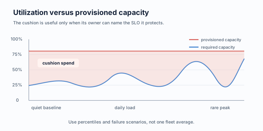
The first accounting mistake is to call all of that area idle. A reserve for one broker failure may be part of the availability design. A reserve for a launch that happens twice a year may be a scheduling candidate. A reserve left over from an incident whose traffic pattern no longer exists is unowned spend. The chart becomes useful only after each band has an owner, a reason, and a removal test.
2Where idle capacity comes from
The same symptom, idle brokers, can have four different causes. Separate them before choosing a scaling policy because each cause changes a different constraint.
| Source of cushion | What it protects | Evidence to collect |
|---|---|---|
| Rare traffic peaks | Throughput and latency during a known event | Peak-to-average ratio, peak duration, producer latency |
| Partition or leader skew | A hot broker hidden by cluster averages | Per-broker network, request rate, leader count, and per-partition traffic |
| Failure and maintenance reserve | Recovery, rolling work, and safe replacement | Recovery test results, reassignment time, and target RTO |
| Storage coupling | The effort and risk of moving durable data | Disk utilization, reassignment volume, and time to restore the former topology |
Rare peaks are a forecasting problem. If the event is predictable, a schedule or a temporary capacity pool may be enough. Skew is a placement problem, so adding brokers without moving leaders or reconsidering partition keys can leave the original bottleneck in place. Failure reserve is a reliability budget and should not be cut because one utilization graph looks comfortable.
Storage coupling is the architectural case. In a traditional Shared Nothing architecture, a broker owns local log segments and participates in replication. Removing that broker can require partition reassignment and data movement before the cluster is safe at the smaller size. The compute may be idle, but the storage ownership is not. That is why a team can be confident that it has spare CPU and still be unwilling to scale in.
Retention and compaction add another boundary. Longer retention increases the data set that must be stored and potentially recovered. Log compaction changes what remains for keyed topics. Neither policy is a reason to keep an arbitrary number of brokers, but both affect the storage and recovery work that a capacity plan must include. Kafka's broker configuration reference is the right place to confirm the retention, replication, and quota settings used in the calculation.
3Measure the cushion in money, not only metrics
The basic calculation is straightforward, but the inputs need discipline:
cushion units(t) = provisioned units(t) - SLO-required units(t)
cushion spend = sum(cushion units(t) x applicable hourly rate(t))
Use the unit that actually drives the charge. It may be broker instances, provisioned storage, provisioned throughput, or a managed service unit. Do not multiply a CPU percentage by an instance price and call the result savings when the cluster is constrained by network, storage, partition count, or recovery time.
A practical worksheet should track at least these fields for each observation window:
- Demand: ingress and egress bytes, request rate, active connections, consumer lag, and the p50, p95, or p99 utilization or traffic percentile that matches the SLO.
- Placement: leaders per broker, partitions per broker, broker network, disk activity, and the hottest partition rather than only cluster totals.
- Safety margin: the failure scenario, recovery target, replication factor,
min.insync.replicas, and the capacity needed while one broker or one failure domain is unavailable. - Cost: broker hours, attached storage, storage performance, object-storage requests or retrieval, and any network charge created by replication or recovery.
Averages are useful for finding the baseline. They are poor evidence for a scale-in decision. Compare the percentile that represents the customer impact with the percentile used in the bill review, then preserve the raw time window so a short burst cannot disappear inside a daily average. Kafka's design documentation explains the replication and partition mechanics that make this comparison necessary.
The second accounting mistake is to ignore the cost of changing capacity. A scale-down that requires a long reassignment window, consumes network bandwidth, or raises recovery risk may not be worth running for a short-lived trough. Add engineering time and rollback risk to the comparison. Conversely, a scale-in that can switch serving capacity without moving the durable data should be evaluated against the same SLO, not rejected because a legacy workflow was expensive.
A capacity cushion is healthy when its owner can state the event, SLO, or failure scenario it protects. It is a tax when the sole justification is that shrinking the fleet feels dangerous.
4Three responses: reserve, schedule, or go elastic
There is no universal Kafka autoscaling setting that makes this decision. The right response depends on the shape of demand and the work required to add or remove a broker.
| Response | Fits when | Main cost or risk | Test before committing |
|---|---|---|---|
| Reserve a fixed fleet | Peaks are frequent, recovery targets are strict, or moving data is expensive | You pay for the trough and may never reclaim the reserve | Name the protected SLO and review it each planning cycle |
| Schedule capacity | Demand follows a reliable calendar and there is time to react to an early peak | A forecast miss can create a saturation event; scale-in still needs a safe path | Run a controlled pre-peak and post-peak transition |
| Use elastic broker capacity | Serving load changes faster than durable data ownership needs to move | Cache, WAL, connections, partition placement, and storage access can become the new limits | Measure add/remove time, client behavior, catch-up reads, and rollback |
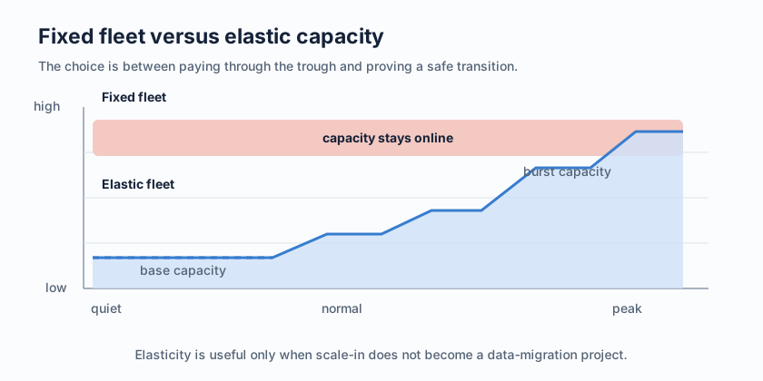
Keeping a fixed fleet is not a failure. It can be the most cost-effective risk-adjusted choice for a payment path with a strict recovery target and an unpredictable peak. The mistake is hiding the reserve inside a utilization dashboard instead of recording it as a deliberate reliability cost.
Scheduled capacity works best when the calendar is stronger than the forecast. It needs a buffer for early starts, a rollback path, and a policy for workloads that do not share the business-hours pattern. It also does not remove the data-movement problem. A scheduled broker that owns local partitions still has to be drained safely when the schedule ends.
Elastic capacity changes the question from "Can we add brokers?" to "What has to move when we add or remove them?" If the answer includes a large durable-data rebalance, the control-plane action may be quick while the actual capacity change remains slow. If the broker is stateless with respect to durable stream data, the scale event can focus on request serving, leadership, cache warming, and recovery checks.
5The architecture test behind elastic brokers
That last distinction gives FinOps and SRE teams a useful architecture test. A candidate platform should be assessed on four separate paths: Kafka protocol behavior, durable storage location, recovery path, and deployment boundary. Kafka compatibility matters because changing the broker should not force every producer and consumer to adopt a new client contract. Storage location matters because a broker-local disk turns compute changes into data movement. The recovery path matters because a shared store does not remove cache, WAL, or object-storage failure modes. The deployment boundary matters because network, IAM, and storage charges still belong to a specific cloud account and Availability Zone (AZ) design.
This is where AutoMQ becomes a candidate for evaluation, after the capacity problem has been made explicit. AutoMQ is a Kafka-compatible cloud-native streaming platform built around a Shared Storage architecture. Its AutoMQ Brokers are stateless with respect to durable stream data, while S3Stream uses WAL storage, data caching, and S3-compatible object storage for the write, recovery, and read paths. In that model, changing broker capacity can be evaluated as a serving-capacity operation instead of assuming that every change requires copying the entire local log set.
The boundary matters. Stateless brokers do not make partition count, connections, request rate, cache size, WAL capacity, or object-storage access disappear. WAL is a write and recovery layer, not long-term primary storage, and the exact behavior depends on whether the deployment uses S3 WAL, EBS WAL, Regional EBS WAL, or NFS WAL. A BYOC (Bring Your Own Cloud) deployment also leaves cloud resource, IAM, storage, and network choices in the customer's account. Those are inputs to the bill, not footnotes.
AutoMQ's Continuous Self-Balancing documentation describes the operational mechanism to examine: balancing serving load across brokers as the workload changes. A proof should measure the real transition, including scale-out time, scale-in time, partition reassignment behavior, client errors, leader movement, catch-up reads, WAL recovery, object-storage requests, and the cost of the chosen deployment topology. A diagram or product setting is not a savings result until those observations line up with the SLO.
6A this-week and this-quarter action list
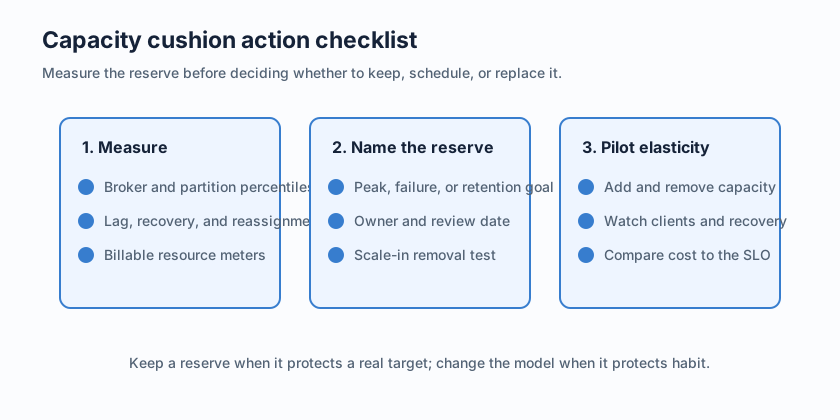
A useful capacity review ends with an owner and a date, not a request to "watch utilization." This week, make the current cushion visible:
- Measure: export a representative window of per-broker CPU, network, request rate, disk activity, partition and leader distribution, consumer lag, and the relevant demand percentiles.
- Name the reserve: attach every extra broker or storage unit to a peak, failure scenario, retention policy, partition-skew fix, or other explicit SLO. Mark unowned capacity separately.
- Price the boundary: use the applicable compute, block storage, object storage, request, retrieval, and network price pages for the region and topology. The AWS EC2 pricing page and AWS EBS pricing page illustrate why the resource meter matters; use the provider's current page for the actual estimate.
This quarter, run one controlled test outside the most sensitive path. A schedule test is enough when the peak is predictable. An elastic-broker test is more informative when storage coupling is the suspected blocker. Record the time to add capacity, the time to remove it, the client and consumer behavior during the transition, the recovery result, and the billable resources that changed.
Then make the decision by scenario. Keep a reserve when the failure or peak objective cannot tolerate a transition. Schedule capacity when demand is predictable and a rollback path exists. Evaluate Shared Storage and stateless brokers when local-data movement is the reason the cushion remains permanent. The outcome may be a smaller fixed fleet, a scheduled fleet, or a different storage model. The important part is that the choice follows evidence instead of habit.
The next time the FinOps review shows 30% average utilization, ask which part of the remaining 70% is protecting a real SLO and which part is paying for an old fear. If the answer is trapped data on broker-local disks, a representative scale test with AutoMQ can turn that fear into measured transition time, recovery behavior, and cost data.
7References
- Apache Kafka design documentation
- Apache Kafka broker configuration reference
- Apache Kafka quotas
- Kafka KIP-405: Tiered Storage
- AWS EC2 On-Demand pricing
- AWS EBS pricing
- AWS S3 pricing
- AutoMQ architecture overview
- AutoMQ Continuous Self-Balancing
8FAQ
8.1Is 30% Kafka utilization proof that the cluster is over-provisioned?
No. Averages can hide hot partitions, short peaks, and failure reserve. Compare per-broker and per-partition percentiles with the SLO, then record why the remaining capacity exists.
8.2What should count as Kafka idle broker cost?
Count the broker or managed-service capacity that remains provisioned during the measured trough. Add attached storage and performance capacity, then include network, recovery, and operational costs that the transition would create. State the region, topology, retention, and time window before comparing totals.
8.3Can Kafka autoscaling remove the capacity cushion?
It can remove part of the reserve when the serving layer can change without an unsafe data migration. It does not remove headroom for partition skew, connections, cache, WAL, recovery, or object-storage limits. Test the transition against the SLO.
8.4When is a fixed Kafka fleet the right choice?
A fixed fleet can be reasonable when traffic is unpredictable, the recovery target is strict, or the cost and risk of moving local data outweigh the idle spend. Treat the reserve as a named reliability budget and review its evidence regularly.
8.5Does Tiered Storage solve idle broker capacity?
Not by itself. Kafka Tiered Storage changes where some historical data is kept, but the serving layer, local state, partition placement, and broker lifecycle still need evaluation. Separate historical retention savings from the cost of keeping brokers online for peak and recovery capacity.