
Table of Contents
Table of Contents
The producer dashboard is flat, but the network line on the cloud bill is not. That is a familiar Kafka inter-AZ traffic cost surprise: logical ingress stayed close to 1 GB, while the same workload generated several gigabytes of eligible movement between Availability Zones (AZs). The extra bytes did not come from nowhere. They came from replica fetches, consumer reads, replay, or a client placement decision that made an otherwise local path cross a billing boundary.
The useful number is not a cluster-wide "Kafka network multiplier." It is a multiplier for a defined workload and a defined boundary. Start with one unit of logical producer data, count each eligible path that carries it, and keep inter-AZ, inter-region, egress, and private-connectivity meters separate. Once the paths are visible, the expensive term usually has an owner and a design choice behind it.
1Inbound flat, network bill up
Kafka metrics describe the stream from the application's point of view. Cloud billing describes movement from the provider's point of view. Those are different measurements even when they refer to the same records. A producer can send 1 GB into a topic, a broker can copy that data to followers, and two consumer groups can each read the full stream. The application sees 1 GB written and 2 GB consumed. The network layer sees a set of paths whose direction, zone placement, and billing treatment may all differ.
The first diagnostic step is to choose a window and stop mixing categories. Use the same hour or day for logical producer bytes, cross-zone flow bytes, and the provider's data-transfer line items. Then ask which behavior changed:
- Replication: Did the leader-to-follower path cross AZs, and did a reassignment or recovery add more copy traffic?
- Consumer fan-out: Are consumer groups in the same AZ as the brokers serving their partitions, or are fetches routinely crossing zones?
- Replay and export: Did a lagging consumer, backfill job, mirror, or cross-region export read the same records again?
This separation matters because each response has a different consequence. Moving consumers can lower a read path without changing durability. Lowering a replication factor changes the failure model. Throttling replay protects a budget but may lengthen recovery.
2The multiplication model: replication, tails, and consumer groups
Let W be the logical bytes written by producers during one measurement window. Define the eligible movement multiplier as:
M = (T_replica + T_consumer + T_replay + T_export) / W
Each T is the byte volume on a path that falls inside the boundary being measured. For an inter-AZ multiplier, count only the cross-AZ portion. For an egress multiplier, use the provider's egress definition. Do not add a producer's inbound bytes to the numerator by default: ingress may be priced differently or not at all, and it is a separate meter.
Replication factor is an upper-bound clue, not the answer. With a replication factor of 3, a partition has one leader and two followers, but the two follower paths may be in the same AZ as the leader, in other AZs, or on a placement that changes during recovery. If both follower fetches cross AZs and each carries approximately the written payload, the illustrative replica term is about 2W. If only one follower path crosses the boundary, it is closer to 1W. Compression, retries, protocol overhead, and partial batches mean the measured value will not match the simple sketch exactly.
Consumer groups add a different term. A group that reads a topic once contributes roughly one stream of read bytes, but only the fraction that crosses the chosen boundary belongs in T_consumer. Two groups with half of their assignments remote can contribute approximately W of cross-zone reads together. A group catching up from an old Offset can read more bytes during the window than producers wrote during that same window, so replay is worth tracking as its own term rather than hiding it inside an average consumer rate.
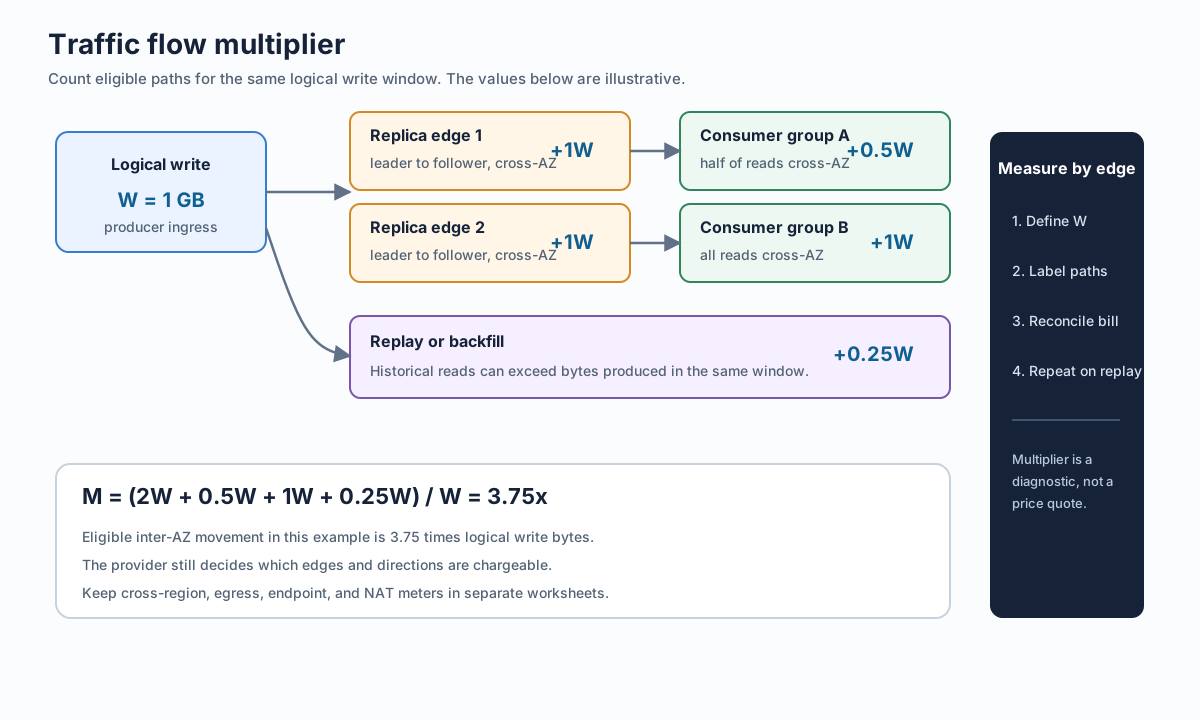
The result is a worksheet, not a promise about a cloud bill. A provider may charge one direction of a path, both sides, or a service-specific transfer category. PrivateLink, NAT, object storage endpoints, and cross-region services can introduce additional meters. The multiplier tells you where to investigate; pricing documentation tells you what a byte on that edge costs.
3A multiplier table for common topologies
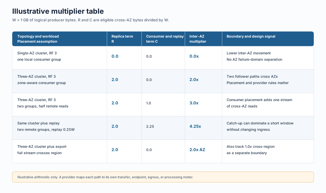
The table below uses an explicitly illustrative workload: W = 1 GB of logical producer data in the window, a replication factor of 3 where noted, and consumer groups that read the full stream. R is cross-AZ replica movement divided by W; C is cross-AZ consumer movement divided by W. The total is a path multiplier for the inter-AZ boundary only. It is not a provider price estimate, and it excludes protocol overhead unless stated otherwise.
| Topology and workload | Replica term R | Consumer/replay term C | Illustrative inter-AZ multiplier | What the row is really saying |
|---|---|---|---|---|
| Single-AZ cluster, three replicas, one local group | 0.0 | 0.0 | 0.0x | Lower inter-AZ movement, but no AZ failure-domain separation. |
| Three-AZ cluster, replication factor 3, zone-aware group | 2.0 | 0.0 | 2.0x | Two follower paths cross AZs in this placement example. |
| Three-AZ cluster, replication factor 3, two groups with half their reads remote | 2.0 | 1.0 | 3.0x | Consumer placement adds one stream of cross-AZ reads. |
Same cluster, two remote groups plus a replay of 25% of W | 2.0 | 2.25 | 4.25x | A short recovery or backfill window can dominate the average. |
| Three-AZ cluster plus a full cross-region export | 2.0 | 0.0 | 2.0x inter-AZ, 1.0x cross-region | One boundary can look stable while another grows. |
These rows are deliberately simple. Real clusters have uneven partition leaders, compression, retries, consumer lag, and different client locations. A 3.0x result does not mean that every provider will charge three times the ingress volume. It means the measured workload contains approximately three units of eligible cross-AZ movement for every unit of logical write, before the provider maps those paths to its own meters.
That distinction keeps the architecture conversation honest. A single-AZ design can make the inter-AZ column look perfect while moving resilience risk into the failure-domain column. Tiered Storage can move older records to object storage while leaving hot data and replica traffic on broker-local storage. A second consumer group can reduce cost when readers are co-located and increase it when assignments are remote.
4Measuring your real multiplier from VPC metrics
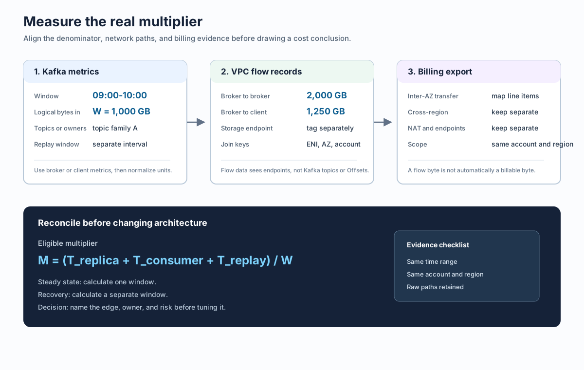
The measurement challenge is attribution. Kafka knows topics, partitions, consumer groups, and Offsets. VPC flow data knows endpoints and bytes. Billing exports know provider categories and charge dimensions. Use them as three aligned slices of one window.
- Choose the denominator. Record producer bytes for the same topics and interval. Broker
BytesInPerSecis a useful starting point for cluster-level work; client metrics are better when you need one application or topic family. Normalize units and account for the fact that compressed client traffic and logical record bytes are not always the same quantity. - Classify the network edges. Aggregate flow records by source and destination interface, subnet, AZ, account, and direction. Label broker-to-broker, broker-to-client, client-to-broker, object-storage, NAT, and private-connectivity paths. Flow records normally cannot identify a Kafka topic or Offset, so join them with client IDs, broker connection data, or workload ownership where that evidence exists. Otherwise, keep the result at the path level instead of inventing topic attribution.
- Reconcile to billing. Compare the classified bytes with the provider's transfer and connectivity line items for the same account, region, and window. Keep inter-AZ, inter-region, Internet egress, endpoint, and NAT categories separate. A mismatch is useful: it may indicate an omitted path, a different aggregation boundary, or a billing rule that does not map one-to-one to flow bytes.
- Repeat under a different workload. Run the calculation for a steady state window and a replay, rebalance, or recovery window. If
Mjumps only during catch-up, the first control is probably replay placement or throttling, not a replication-factor change.
The output is a small table with W, T_replica, T_consumer, T_replay, T_export, the path owner, and the applicable provider meter. Keep raw evidence beside the calculation. When finance asks why network spend grew while ingress did not, point to a path and a change rather than a monthly total.
5What lowers the multiplier, and what does not
Some changes reduce a term without changing the storage architecture. Place consumers with the partitions they read when the application can tolerate that constraint. Use batching and compression where the workload and latency target allow it. Cap replay concurrency, schedule backfills away from budget-sensitive windows, and make cross-region exports explicit. These controls reduce bytes or change their route, but they do not remove broker-to-broker replication from a Shared Nothing architecture.
Other changes alter the failure boundary. Adding AZs can improve availability while creating more possible replica and fetch edges. Dropping a replica can reduce movement while weakening redundancy. Pinning all clients to one zone can reduce the bill and concentrate a failure domain. Private connectivity can improve routing and security while adding endpoint or processing charges. Each proposal should name the edge it removes and the risk or new meter it introduces.
This is also where Tiered Storage needs careful wording. Apache Kafka's KIP-405 model moves older data to remote storage while retaining a local tier for recent data. It can change retention economics and historical-read behavior, but it does not automatically turn a multi-AZ broker cluster into a single-copy network model. If the largest term is hot-data replication between broker-local disks, moving cold data is aimed at a different term.
The architecture question is narrower than "How do we reduce Kafka cost?" Which durable copy or read path is creating the movement, and can that boundary move without losing the required failure objective?
6When the storage boundary is the multiplier
If the dominant term is broker-local replica movement, the next option is a storage architecture that does not require each broker to own a durable copy of the stream. A qualifying design needs more than object storage in a diagram. Check the write acknowledgment path, recovery path, read path, object-storage endpoint placement, WAL behavior, client compatibility, and which traffic remains billable.
AutoMQ is a Kafka-compatible cloud-native streaming platform that uses a Shared Storage architecture. Its S3Stream layer writes durable stream data to S3 storage, while brokers handle Kafka requests, routing, caching, and scheduling. WAL provides a write and recovery layer, so the exact latency and failure boundary still depend on the selected WAL type and deployment model.
That design changes the replica term rather than magically deleting every network cost. In an applicable S3-backed deployment, durable data is not maintained as broker-local copies that need the traditional leader-to-follower path across AZs. Tailing Read may be served from cache or WAL, while Catch-up Read can fetch historical data from S3 storage. There is no follower replica edge for those reads, but there can still be object-storage requests, client-to-broker movement, cross-zone endpoints, and egress. AutoMQ's Zero cross-AZ traffic documentation describes the supported routing design; validate the actual deployment, endpoint path, and provider meter before using the claim in a budget.
WAL choice matters. AutoMQ Open Source uses S3 WAL, while AutoMQ commercial editions can support other WAL storage types such as Regional EBS WAL and NFS WAL. A Regional EBS WAL can change the persistence and network boundary again, so a comparison should identify the product version, WAL type, AZ placement, and object-storage path. Treat "replication multiplier becomes 1" as a model for the durable storage edge, not as a claim that the complete workload costs one unit of network traffic.
7Scenario guidance: choose the term you need to change
The right intervention depends on what the measurement shows:
- Replica movement dominates: compare a Shared Storage architecture with the current broker-local design. Preserve the required durability and recovery objectives, then model object storage, WAL, and endpoint charges.
- Consumer reads dominate: fix locality first. Move clients, use zone-aware assignment where appropriate, or decide whether the latency and availability trade-off of local reads is acceptable.
- Replay dominates: treat catch-up as a workload with a budget. Control concurrency and measure the recovery window separately from steady state.
- Cross-region export dominates: price the destination and replication schedule directly. Reducing inter-AZ movement in the source cluster will not remove a cross-region copy.
Return to the original surprise: flat ingress and a rising network bill are compatible because ingress is only the first edge. To test your own workload, start with AutoMQ and bring the measured topology, not just the bill.
8References
- Apache Kafka design
- Apache Kafka broker configurations
- Apache Kafka consumer configurations
- Kafka KIP-405: Kafka Tiered Storage
- AWS VPC Flow Logs
- AWS VPC pricing
- AWS data transfer pricing
- AutoMQ Shared Storage architecture
- AutoMQ Zero cross-AZ traffic
9FAQ
9.1What is the Kafka inter-AZ traffic multiplier?
It is the ratio of eligible cross-AZ bytes to logical producer bytes for a defined workload and time window. Replication, consumer reads, replay, and exports can each contribute. It is not a fixed Kafka property or a universal cloud pricing factor.
9.2Does replication factor equal the network multiplier?
No. Replication factor tells you how many copies a partition is configured to maintain. The network multiplier depends on where those copies sit, which paths cross the boundary, and whether recovery or reassignment is active. Provider billing rules determine which of those bytes become chargeable.
9.3Can zone-aware consumers make the multiplier zero?
They can reduce consumer fetch movement when readers and the brokers serving their partitions are co-located. They do not remove cross-AZ replica traffic in a traditional multi-AZ Shared Nothing cluster, and assignments can change during rebalances or failures.
9.4Does shared storage eliminate Kafka network costs?
No. It can remove a broker-local replication term in an applicable architecture. Consumer paths, object-storage access, WAL, replay, egress, private connectivity, and cross-region movement still need to be measured and priced separately.
9.5What should a FinOps review ask for first?
Ask for the denominator and the boundary: logical producer bytes for a named window, eligible bytes by path, the consumer and replay workload, and the provider line items mapped to those paths. Without those four pieces, a multiplier is only a suspicion.