
Table of Contents
Table of Contents
The budget meeting started with a familiar question: should the team buy more broker capacity for a rising Apache Kafka workload, or move more of its budget into storage? The platform team had a throughput graph. FinOps had a storage forecast. Both were correct, but they were measuring different clocks.
That distinction matters. A short traffic burst can force more compute capacity without materially changing retained history. A retention request can multiply stored bytes while the peak producer rate stays flat. Kafka throughput cost and Kafka storage cost belong in the same model, but they should not be treated as the same meter.
The estimate below uses a hypothetical 100 MB/s workload and clearly labeled illustrative rates. It is a reusable capacity model, not a provider quote. Replace the rates with the current price for your region, storage class, broker or capacity unit, network path, and deployment model before using it for procurement.
1One workload, two very different bills
Throughput is a rate. Storage is a quantity accumulated over a retention window. The first usually follows the peak service envelope: producer rate, consumer rate, partition count, connections, request size, batching, and the headroom needed for failures or maintenance. The second follows the bytes that survive long enough to be retained, after compression, compaction, replication or erasure layout, and cleanup lag have been applied.
Workload shape decides which one moves first. Consider three streams with the same seven-day retention:
- A telemetry stream writes steadily and has few historical reads. Its broker capacity may be predictable, while retained storage grows almost directly with ingress.
- A clickstream is quiet most of the day but has a sharp peak during campaigns. Its peak compute and network envelope can dominate even when average retained volume is moderate.
- A CDC stream has a modest write rate but several consumers that replay old offsets. Its stored bytes may be manageable, yet catch-up reads, cache pressure, and retrieval requests can become the expensive part.
These are not three pricing products. They are three different shapes applied to the same pricing dimensions. A broker-hour, a capacity unit, a provisioned throughput tier, an object request, or a data-transfer line can be the provider's actual billing unit. The first task is to map each provider line to the work that created it.
The Apache Kafka design documentation is useful here because it keeps the system mechanics separate: producers and consumers create request work, while retention and replication determine how long and how many copies of data remain in the cluster. The bill follows those mechanics, plus the provider's own pricing boundaries.
2Writing throughput and storage as one equation
Start with two terms instead of one vague "Kafka cost per MB/s" number. Let W be effective logical ingress in decimal MB/s, T be the retention window in seconds, and P be the physical-storage multiplier after compression, replication, segment overhead, and any storage layout. The retained storage quantity is:
logical retained GB = W × T ÷ 1,000
physical retained GB = logical retained GB × P
P is where teams often hide a major assumption. If each logical byte is compressed to 0.6 physical bytes on each of three replicas, P is 1.8. If a shared-storage design keeps one durable object copy and a separate WAL or cache, its physical multiplier is different. Do not carry a replication factor from one architecture into another without checking what that factor means at the storage boundary.
The monthly model can then be written as:
monthly cost = throughput envelope
             + physical retained GB × storage rate
             + network transfer
             + request and retrieval charges
             + WAL, cache, and operational capacity
The throughput envelope is intentionally broad. A managed Kafka service may express it as broker-hours or capacity units instead of a per-throughput rate. For comparison, normalize that line to a monthly cost for the required peak workload, but keep the original provider unit in the worksheet. Do the same for storage: use the provider's billable GB-month definition, not a raw disk-size estimate.
The following unit table is a practical starting point. The numbers are illustrative inputs for the worked estimate, not current prices from a cloud provider.
| Meter | What drives it | Illustrative input | Calculation | Boundary to verify |
|---|---|---|---|---|
| Throughput envelope | Peak producer and consumer service capacity | $25 per sustained MB/s-month | 100 × $25 = $2,500/month | Broker-hours, capacity tiers, connections, and peak headroom may replace this meter |
| Retained storage | Physical bytes kept for the retention window | $0.08 per GB-month | Physical GB × $0.08 | Region, volume type, object class, and provisioned versus used capacity |
| Network and requests | Replication, client paths, reads, and API calls | Excluded from the base case | Add measured GB and request counts | AZ direction, egress, retrieval, and request pricing vary by provider |
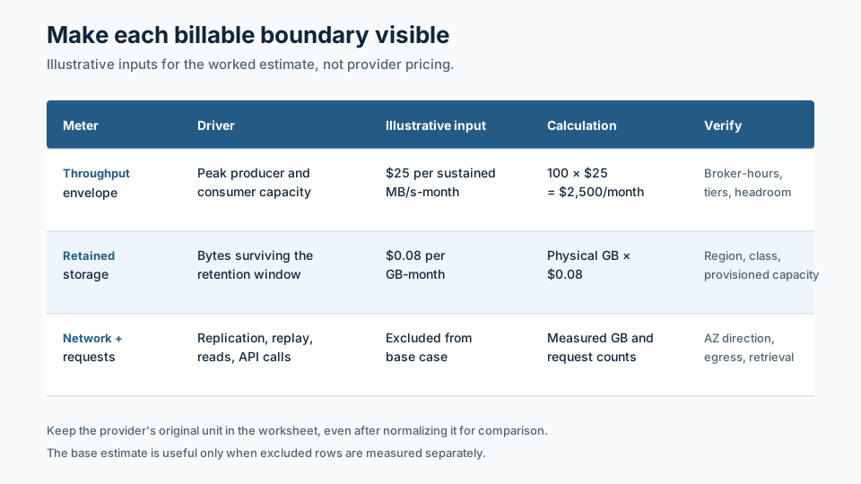
The table makes an important limitation visible. A storage-only comparison can look favorable while request, replay, or AZ (Availability Zone) traffic changes the result. Conversely, a broker-heavy comparison can overstate the value of a storage redesign when peak partitions or consumer fan-out are the real constraint.
3A worked estimate: 100 MB/s for seven days
Use a steady 100 MB/s of logical ingress, seven days of retention, a physical multiplier of 1.8, and the illustrative storage rate of $0.08 per GB-month. Assume the peak throughput envelope is unchanged across the retention scenarios and normalize it to $2,500 per month.
First calculate the logical bytes:
100 MB/s × 604,800 seconds ÷ 1,000 = 60,480 GB
Seven days of this workload produces 60.48 TB of logical retained data. Applying the illustrative physical multiplier gives:
60,480 GB × 1.8 = 108,864 physical GB
108,864 GB × \$0.08 = \$8,709.12/month
The base case is therefore:
| Cost line | Formula | Illustrative monthly result |
|---|---|---|
| Throughput envelope | 100 MB/s × $25 | $2,500 |
| Retained storage | 100 MB/s × 7 days × 1.8 × $0.08/GB-month | $8,709 |
| Network, requests, retrieval | Not modeled | Add from provider and telemetry data |
| Base total | Throughput + storage only | $11,209 |
Storage represents about 78% of the modeled total. That is the point of the example, not a claim about every Kafka cluster. The percentage comes from the chosen rate, physical multiplier, and retention window. Change any of those and the balance moves.
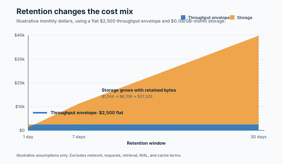
The estimate is also sensitive to what 100 MB/s means. If it is already compressed wire traffic, the logical-to-physical calculation needs a different input. If it is an average and the peak is 300 MB/s, the throughput envelope may require more brokers or capacity units even though retained bytes still grow from the average. If the topic has a replication factor of three but consumers read from a different AZ, network is a separate multiplier, not part of the storage number.
4Retention changes both the total and the balance
Hold the rate, physical multiplier, storage price, and throughput envelope constant. Change retention. The storage term grows linearly because each extra day adds another day's bytes; the throughput term stays flat because this example assumes the same peak and the same capacity plan.
| Retention | Logical retained data | Physical retained data at 1.8x | Storage cost | Modeled total | Storage share |
|---|---|---|---|---|---|
| 1 day | 8,640 GB | 15,552 GB | $1,244 | $3,744 | 33% |
| 7 days | 60,480 GB | 108,864 GB | $8,709 | $11,209 | 78% |
| 30 days | 259,200 GB | 466,560 GB | $37,325 | $39,825 | 94% |
At one day, the normalized throughput line is the larger part of the base model. At seven days, storage dominates. At thirty days, the two lines have not traded places because of a clever pricing trick. Retention has added 25.9 days of physical bytes while the peak service requirement has not changed.
The real system may not behave as cleanly. Longer retention can increase segment count, metadata, compaction work, cache misses, object requests, and historical reads. Shorter retention can shift data into an external archive and add retrieval or egress charges. Kafka's retention.ms and retention.bytes topic settings define deletion constraints, but they do not tell you the provider's full storage or network bill.
That is why a useful capacity model has at least two sensitivity axes. Vary retention to expose storage risk. Vary peak ingress, consumer fan-out, and replay rate to expose throughput and access risk. Then add the network and request rows that the base case intentionally excluded.
5Which one dominates, and what to do about it
The dominant meter should determine the first question, not the first architecture you happen to know. Use the following rules as a triage card:
- Throughput dominates: compare peak-to-average rate, partition skew, request size, batching, connection count, consumer fan-out, and failure headroom. A storage migration will not fix a partition or network bottleneck.
- Storage dominates: verify retention by topic, compression, physical replication, cleanup lag, and how much broker-local capacity is provisioned but unused. This is where separating durable storage from broker compute becomes a credible architecture question.
- Network or access dominates: measure replication direction, cross-AZ placement, replay volume, object requests, and egress. A lower storage rate can lose its benefit if historical reads create a large retrieval bill.
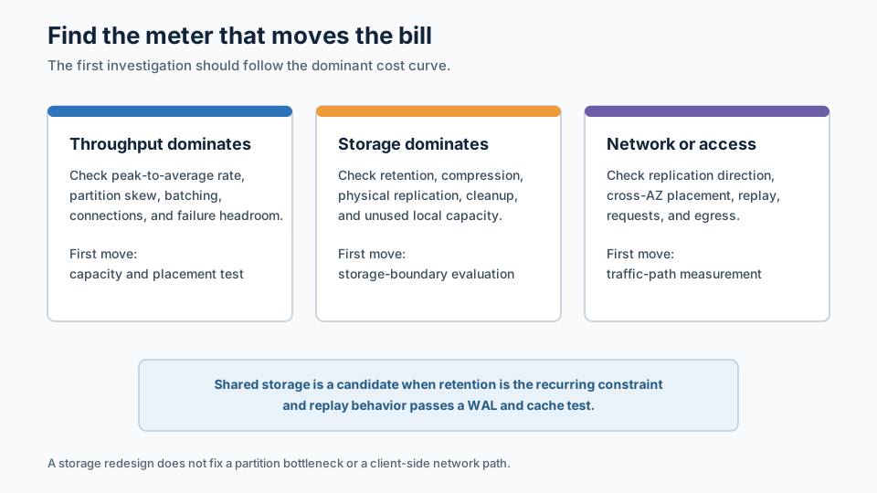
The architecture requirement follows from that diagnosis. For a throughput-dominated workload, the candidate may be better partition placement, producer batching, quota tuning, or a service tier with more predictable peak capacity. For a storage-dominated workload, the candidate may be shorter retention, log compaction, a Tiered Storage design, or shared durable storage. Those choices are not interchangeable: Apache Kafka Tiered Storage, for example, adds a remote log tier while retaining a local tier, so its local capacity, handoff behavior, remote reads, and request charges still belong in the model. The distinction between a local-plus-remote tier and a shared durable storage boundary is also covered in this Kafka compute and storage separation guide.
If the requirement is Kafka-compatible access with durable retention that is not tied one-for-one to broker-local disk, AutoMQ is one architecture to evaluate. Its Shared Storage architecture keeps the Kafka protocol and semantics at the client boundary while using S3Stream, WAL storage, caching, and S3 storage for the persistence path. The architecture overview explains the separation between AutoMQ Brokers and durable storage.
That separation changes the shape of the estimate, not the existence of a bill. The storage row can move from provisioned broker-local volumes to object storage, while the worksheet gains WAL, cache, object requests, catch-up reads, and egress terms. The selected WAL type also matters. S3 WAL, Regional EBS WAL, and NFS WAL have different latency, durability, and price boundaries; treat "WAL" as a placeholder until the deployment model is known. The WAL storage documentation describes that boundary.
For a BYOC (Bring Your Own Cloud) deployment, the cloud account, VPC (Virtual Private Cloud), region, object-storage class, and network path remain part of the customer's estimate. AutoMQ's documented Zero cross-AZ traffic behavior applies to the relevant shared-storage traffic path, not to every client, connector, retrieval, or egress flow. Validate the actual path with provider billing data and workload telemetry. The same discipline applies to a broader Kafka cost model worksheet: keep capacity, storage, network, and operational assumptions visible.
The practical decision rule is narrow: choose a shared-storage candidate when retained history is the recurring constraint, broker-local storage is forcing capacity decisions, and replay behavior can be tested against the selected WAL and cache. Keep the current model when peak throughput, low-latency tailing, or cross-system network paths dominate. In both cases, run the same inputs through the same worksheet so the architecture changes one boundary at a time.
Back at the budget meeting, the platform team can now answer the original question without choosing a side by intuition. The seven-day case is storage-heavy under the stated assumptions; a one-day case is not. That is the useful result: not a universal Kafka price, but a calculation that shows which assumption is making the bill move.
If your own estimate points to long retention and broker-local storage as the limiting boundary, run the same model with AutoMQ, using your measured ingress, peak, retention, replay, WAL, object-storage, and network inputs.
6References
- Apache Kafka design documentation
- Apache Kafka topic configurations
- Apache Kafka KIP-405: Kafka Tiered Storage
- Amazon EBS pricing
- Amazon S3 pricing
- AutoMQ architecture overview
- AutoMQ WAL storage
7FAQ
7.1Is Kafka throughput cost the same as broker cost?
No. A provider may bill broker-hours, capacity units, provisioned throughput, requests, or another service-specific unit. Broker cost is one way to express the throughput envelope, but peak partitions, connections, consumer fan-out, network, and headroom can change the required capacity.
7.2How do I calculate Kafka storage cost per MB/s?
Convert the rate into retained bytes first: MB/s × retention seconds ÷ 1,000 gives decimal GB. Multiply by the physical-storage factor, then by the provider's billable GB-month rate. Keep compression, replication, cleanup lag, and storage class explicit instead of hiding them inside one unexplained multiplier.
7.3Does longer Kafka retention always make storage the dominant cost?
No. It does so in the worked example because the illustrative storage rate and physical multiplier make the storage curve steeper than the normalized throughput line. A low-ingress workload, a high-throughput service tier, or large replay and network charges can produce a different result.
7.4When should I evaluate shared storage?
Evaluate it when durable history, broker-local volume provisioning, or storage-driven scaling is the recurring constraint. Include WAL, cache, object-storage requests, historical reads, egress, and failure recovery in the comparison. A shared-storage design is not a reason to omit access-pattern testing.