
Table of Contents
Table of Contents
Object storage changes Kafka economics, but it does not make storage cost one-dimensional. A WarpStream cost model that only multiplies retained bytes by an S3, Google Cloud Storage, or Azure Blob Storage capacity rate will miss the part of the bill shaped by API operations, read locality, compaction, retention scans, and replay behavior.
That distinction matters because WarpStream is built as a diskless, Kafka-compatible streaming platform on cloud object stores. Its public architecture documentation describes stateless Agents that write data to object storage and coordinate with a metadata store. Its billing documentation also separates WarpStream commercial meters such as cluster-minutes, uncompressed GiB written, and uncompressed GiB stored from the customer's underlying cloud infrastructure in BYOC deployments. The buyer therefore has two related questions: what does WarpStream meter, and what does the cloud object store meter underneath the workload?
The useful answer is workload-specific. Object storage is attractive because durable capacity can be decoupled from broker-local disks, and because object stores are designed for high durability and elastic capacity. The harder FinOps problem is estimating how many objects and requests a Kafka workload creates when producers, consumers, retention policies, and replay jobs meet a real architecture.
1Why Object Storage Cost Is More Than GiB-Month
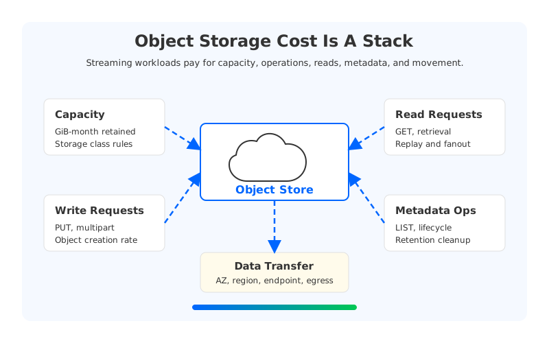
Cloud object storage pricing usually has at least four layers. The first is retained capacity, often expressed as GB-month or GiB-month. The second is operations: writes, reads, lists, lifecycle transitions, metadata operations, and retrieval requests. The third is data movement, including egress, inter-region transfer, or private connectivity depending on placement. The fourth is storage class behavior, where a lower capacity rate can come with retrieval charges, minimum storage duration, or different operation pricing.
AWS S3 pricing is explicit about this split: customers pay for storage and for requests made against buckets and objects, with request categories such as PUT, COPY, POST, LIST, GET, SELECT, lifecycle transition, and retrievals. Google Cloud Storage similarly distinguishes Class A operations, Class B operations, and free operations. Azure Blob Storage pricing separates storage capacity from operations and data retrieval behavior across access tiers.
For streaming systems, this matters because the storage engine is not writing a single monthly archive file. It is continuously turning Kafka records into durable objects, then serving tailing reads, catch-up reads, replays, and retention cleanup. A workload with steady writes and one tailing consumer group can have a very different request profile from a workload with dozens of consumer groups, frequent offset rewinds, and long retention for analytical replay.
A practical model should separate these variables:
- Capacity: retained logical data, retained physical objects, replicas or regions, and storage class.
- Write operations: object creation rate, multipart behavior, metadata commits, and compaction output.
- Read operations: hot reads, cache misses, cold replays, historical scans, and consumer fanout.
- List and metadata operations: retention discovery, compaction planning, object indexing, and operational tooling.
- Data transfer: client placement, object store endpoint placement, cross-region recovery, and private network paths.
The key point is not that object storage requests always dominate the bill. Often they do not. The point is that request sensitivity is workload-dependent, and that sensitivity is exactly what a proof of concept should measure before a platform decision.
2Workload Variables That Drive Request Cost
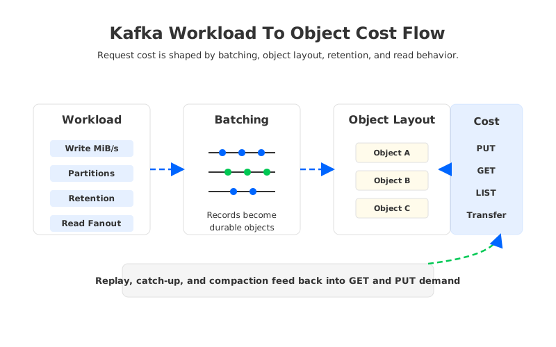
Kafka workloads create object storage cost through shape, not only volume. Two teams can both write 50 MiB/s and retain seven days of data, yet land on different object storage bills if one has small topics with high partition count and frequent catch-up, while the other has fewer hot topics with stable tailing reads.
| Workload variable | Cost mechanism | What to measure |
|---|---|---|
| Average write throughput | Retained data and object creation | MiB/s, compressed and uncompressed basis |
| Partition count | Object locality and metadata scale | Partitions per topic and active partitions |
| Batch size and object size | PUT count and GET efficiency | Objects per GiB written, average object size |
| Retention by topic class | Stored GiB-month and deletion work | Hours or days per topic family |
| Consumer fanout | Fetch volume and cache pressure | Groups, replay jobs, and read/write ratio |
| Cold replay frequency | GET requests, retrieval, and network | Rewinds per week and bytes replayed |
| Compaction behavior | Extra reads/writes in exchange for locality | Compaction cadence and output object count |
2.1Write Batching and Object Size
Object size is the bridge between streaming write behavior and object storage request economics. If a system writes many tiny objects, PUT and metadata overhead can rise, and later reads may need more object fetches. If it waits too long to create larger objects, end-to-end latency and buffering requirements can suffer. The design problem is a tradeoff, not a one-way optimization.
WarpStream's write path documentation describes batching data into files in object storage and then using background file compaction. It says compaction can merge batches for the same topic-partition from different files, improve IO access patterns for historical replays, and reorganize data to improve locality. Its architecture page also frames batching and compaction as a tradeoff between cost and end-to-end latency.
That is the right place to ask for PoC evidence. Do not ask only for a headline request reduction. Ask for objects per TiB written, average object size, compaction input and output bytes, and the number of PUT, GET, and LIST-like operations during steady ingest. Those counters tell you whether the architecture is using object storage as a large-object system or accidentally turning it into a high-churn metadata surface.
2.2Retention and Cold Reads
Retention is usually modeled as capacity, but it also changes read cost. A seven-day operational retention window with mostly tailing consumers is not the same as a 30-day or 90-day replay window used by analytics, incident investigation, or model feature backfills. Longer retention expands the cold surface area: more objects remain eligible for historical reads, lifecycle transitions, and cleanup.
The first sizing formula is still useful:
retained GiB = average write MiB/s x 3600 x retention hours / 1024
For example, a workload writing 40 MiB/s with 168 hours of retention has a logical retention anchor of about 23,625 GiB before compression, implementation overhead, and multi-region copies:
40 x 3600 x 168 / 1024 = 23,625 GiB
That number is not a quote. It is the denominator for better questions. How many physical bytes are stored in the cloud bucket? Are WarpStream storage meters based on uncompressed logical GiB while the cloud bucket stores compressed physical objects? Does retention cleanup scan object metadata? Are older objects in a storage class with retrieval charges or minimum duration? Are replay reads served from cache, local disk, or direct object storage GET operations?
2.3Consumer Fanout and Catch-Up Reads
Read fanout is where object-storage-backed Kafka cost models often become too optimistic. Tailing consumers may read data while it is still hot in memory or cache. Lagging consumers, new applications, disaster recovery drills, and backfills may read older data that has aged out of the hot path. The same retained byte can be cheap if it is never revisited and more expensive if it is replayed repeatedly by independent consumers.
WarpStream's read path documentation says Agents maintain a per-Availability Zone cache that behaves like a distributed mmap and decouples the number of partitions and consumers from the number of object storage GET requests needed to serve Kafka Fetch requests. That is an important design claim, and it should be tested with the buyer's workload rather than assumed from a small demo.
Use at least three read scenarios in the evaluation: steady tailing consumption, one large catch-up after consumer downtime, and a planned historical replay. Measure cache hit behavior, object storage GET requests, read latency, network transfer, and whether one replay disrupts tailing consumers. This will show whether the cost model is stable under normal operations and during the events that usually expose hidden cost.
3What To Measure In A WarpStream Evaluation
A WarpStream object storage evaluation should produce cloud-provider counters, not only application throughput charts. The architecture intentionally moves durable bytes into object storage, so the bucket, network, and Agent fleet are part of the measurement surface.
Start with the following measurement plan:
- Normalize bytes. Record compressed producer bytes, uncompressed logical bytes, retained logical GiB, and physical bucket growth separately.
- Track object operations. Capture PUT, GET, LIST or equivalent operations, lifecycle requests, and delete activity during steady ingest, catch-up, and retention cleanup.
- Observe object layout. Record object count, average object size, small-object percentage, and compaction output over time.
- Test read locality. Compare tailing reads, consumer lag recovery, and historical replay for request volume and latency.
- Map network paths. Identify client-to-Agent, Agent-to-object-store, cross-AZ, cross-region, and private connectivity charges.
- Add failure cases. Restart Agents, remove capacity, throttle a dependency where safe, and measure whether requests or reads spike.
The resulting model should have sensitivity columns. Change retention from seven days to 30 days. Change read fanout from 1x to 5x. Add one daily replay job. Increase partition count. Move from single-region to multi-region. The architecture may still be attractive under all those cases, but the budget owner should know which variable bends the curve.
Confluent's September 2024 WarpStream acquisition announcement positioned it as a BYOC streaming option for large-scale workloads with relaxed latency requirements, including logging, observability, and feeding data lakes. Those workloads are often storage-heavy, replay-sensitive, or both. A buyer should validate the object storage profile with representative retention and read behavior, not with a generic Kafka benchmark.
4How AutoMQ Manages Object Storage Economics
The broader category is Kafka-compatible streaming on shared object storage. WarpStream is one implementation in that category. AutoMQ is another: it keeps Kafka protocol compatibility while using S3-compatible object storage as the durable storage layer, with stateless brokers and an S3Stream storage design. That makes it relevant to the same object storage cost conversation, but the comparison should stay architectural and measurable rather than promotional.
AutoMQ's S3 storage documentation describes two object types in S3Stream. A Stream Object stores data for an individual stream, while a Stream Set Object consolidates smaller streams when WAL data is uploaded. The same documentation describes background compaction that merges smaller objects to reduce metadata scale, and the broker configuration documentation exposes compaction-related settings where larger values can reduce API call cost but change metadata or compaction tradeoffs. AutoMQ also documents the WAL as a write acceleration and fault recovery path while S3 remains the actual storage location for data.
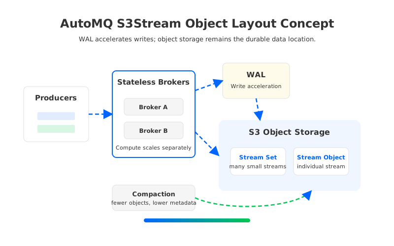
This gives platform teams a concrete comparison framework. For WarpStream, ask how batching, file compaction, distributed cache, and retention cleanup affect object count and GET volume. For AutoMQ, ask how WAL, Stream Set Objects, Stream Objects, compaction interval, compaction cache, and read caching affect the same counters. For traditional Kafka, ask how broker-local disks, replication factor, segment retention, and partition reassignment shape disk, network, and operating cost.
The right answer depends on workload. Append-heavy telemetry with long retention may reward a different object layout than low-latency transactional streams with high fanout. A replay-heavy analytics workload should care more about cold-read locality than a simple log pipeline.
5Object Storage Cost Checklist
Use this checklist before accepting any object-storage-backed Kafka estimate:
- Byte basis: Are written and stored units compressed, uncompressed, logical, or physical?
- Request basis: How many PUT, GET, LIST, lifecycle, and delete operations are expected per TiB written and per TiB replayed?
- Object layout: What is the average object size, and how does compaction change it over 24 hours?
- Retention classes: Which topics retain data for hours, days, weeks, or months?
- Read pattern: What percentage of reads are tailing, lag recovery, historical replay, or analytical scan?
- Cache behavior: Which reads hit memory, local cache, distributed cache, WAL, or object storage?
- Network path: Which paths are same-AZ, cross-AZ, cross-region, internet egress, or private connectivity?
- Failure mode: What happens to object requests during node replacement, Agent restart, zone impairment, or object store throttling?
- Cloud ownership: Which costs appear on the vendor invoice, and which appear in the customer's cloud account?
The most useful object storage model is not the one with the most precise first estimate. It is the one that tells you where precision is still missing. If request counts are unknown, measure them. If replay behavior is uncertain, replay real data. If retention varies by topic, model topic classes instead of one average. Object storage can be a strong foundation for Kafka-compatible streaming, but only when the cost model treats it as an active data plane rather than a passive bucket.
6References
- WarpStream Architecture
- WarpStream Write Path
- WarpStream Read Path
- WarpStream Billing Reference
- WarpStream Pricing
- AWS S3 Pricing
- Google Cloud Storage Pricing
- Azure Blob Storage Pricing
- Apache Kafka Documentation: Log Compaction
- Confluent Acquires WarpStream
- AutoMQ S3 Storage Documentation
- AutoMQ Broker and Controller Configuration
7FAQ
7.1Is WarpStream object storage cost only S3 storage capacity?
No. Capacity is only one part of the model. In BYOC deployments, the customer cloud account can also see object storage requests, data transfer, compute for Agents, private connectivity, logs, metrics, and other infrastructure charges. WarpStream's own billing dimensions are separate from those cloud-provider charges.
7.2Which S3 requests matter most for Kafka-style workloads?
PUT and GET requests are usually the first categories to examine because streaming systems continuously write objects and serve reads. LIST, lifecycle transition, retrieval, and delete-related behavior can also matter depending on object layout, retention cleanup, storage class, and operational tooling.
7.3Why do read patterns affect object storage cost?
Tailing reads may be served from hot paths or caches, while catch-up reads and historical replay may touch older objects. High fanout, frequent offset rewinds, and analytical scans can increase GET requests, network transfer, and cache pressure even when write volume is unchanged.
7.4How should I compare WarpStream and AutoMQ on object storage economics?
Use the same workload and measure the same counters: written bytes, retained bytes, object count, average object size, PUT/GET/LIST operations, cache hit behavior, compaction output, network paths, and recovery behavior. Then compare how each architecture changes those counters.
7.5What is the fastest way to validate the estimate?
Run a proof of concept with production-like write rate, partition count, retention classes, and read fanout. Include at least one lag recovery test and one historical replay. Export cloud-provider object storage metrics and vendor billing counters into the same worksheet.