
Table of Contents
Table of Contents
A pricing page will tell you exactly what a broker-hour costs, what a retained gigabyte costs, and what a gigabyte of cross-zone transfer costs. It will not tell you what one byte costs, because the honest answer depends on what that byte is doing: being written for the first time, sitting on disk for fourteen months, traveling between zones as a replica, or being re-read by a consumer that is catching up after an incident.
That is why two teams with comparable workloads can look at the same vendor quote and reach opposite conclusions about whether it is expensive. They are pricing different bytes without saying so.
1The question pricing pages avoid
Think of a single event entering a topic: a request log line, a sensor reading, a payment record. From the moment the producer writes it, that record starts accumulating cost across several independent services, and each service meters it differently.
It costs money to hold the record on durable storage for as long as retention requires. It costs money to move it across network paths that its own producer never sees, such as replication traffic between brokers or retrieval from a remote tier. It costs money to keep CPU scheduled so the broker, controller, and connectors exist at all, whether the current second is busy or idle. It costs money again when the record makes a trip that looks free, such as a consumer replaying a day of history.
Most pricing pages answer these questions separately, because each answer is a separate line item. The difficult part is assembling the lines into one number that two vendors can be compared against. The difference between an honest comparison and a misleading one is whether those lines are ever assembled into one per-byte figure.
2Storage, network, compute: three meters for one byte
The simplest honest model is three meters attached to the same byte: storage measures how much data remains and for how long; network measures how many billable boundaries the byte crosses; compute measures how much capacity is reserved to do all of it.
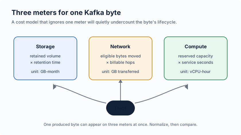
Storage is easiest to reason about when its unit is the retained GB-month: the amount of data kept, times the number of months it sat there. A platform that prices per GB-month is already using this unit. One that prices per broker-hour is not: it is charging you for the disks attached to the brokers, which means you pay for capacity provisioned, not capacity used.
Network deserves the same precision. A byte traveling from a producer to a broker is traffic; the same byte replicating to two other brokers is more traffic; the same byte fetched by five consumer groups is traffic again. Whether any given hop is billable depends on zone placement and the provider's data transfer rules, which is exactly why "network" must stay a separate meter rather than being folded into "storage" or "compute."
Compute is the meter people set by feel. A broker fleet is usually sized to a peak, then left running through the trough. When the per-byte question comes up, idle compute shows up as a real cost per delivered byte, even though it consumed no bytes at all.
| Meter | Natural unit | What it actually captures |
|---|---|---|
| Storage | GB-month | Retained data, replicas, remote tiers, time |
| Network | GB transferred | Every billable hop the byte crosses |
| Compute | vCPU-hour or service-hour | Reserved capacity, not just work done |
3Normalizing vendor units to a common scale
Different vendors quote different units because each unit hides a different assumption. One quotes a broker-hour and leaves storage utilization to you. Another quotes a throughput quota and leaves partition count to you. A third quotes object storage plus requests and makes you assemble the write path yourself.
The way to compare them is to force every quote onto a denominator your own workload defines. Decide whether the denominator is logical GB produced, retained GB-month, or GB delivered to consumption, then convert each vendor's unit into that denominator before anyone touches a calculator.
normalized cost = eligible monthly cost / chosen workload denominator

acceptable denominators:
- logical GB produced
- retained GB-month
- GB delivered to one consumer group
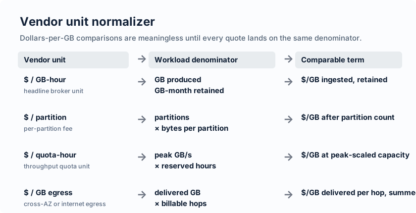
The conversion itself is arithmetic. A GB-hour figure needs an assumption about how many broker-hours serve how many produced, retained, and delivered gigabytes during a month. A per-partition fee needs a partition count and a bytes-per-partition estimate before it means anything per byte. A throughput quota needs a peak-to-average ratio and the number of reserved hours; a fleet sized for a yearly peak prices every average-traffic byte at peak rates.
What makes the comparison fall apart is not the math but ambiguity in the word "GB." A compressed producer byte, an uncompressed broker byte, and a retained-replica byte are three different quantities. State the unit before comparing, and record how it was derived, or the numbers were never comparable in the first place.
4The multipliers hiding in replication, retention, and access patterns
Once the meters are separated, the same workload can be re-priced by changing three multipliers. Replication multiplies movement and storage: a topic configured with a replication factor above one keeps copies on multiple brokers, and min.insync.replicas turns that durability choice into an availability floor. Retention multiplies storage: the same ingest rate fills many months of disk, and Apache Kafka's log retention settings determine when segments can finally be deleted. Access patterns multiply network and compute: fan-out, catch-up reads, and compaction can make read and rewrite traffic larger than the producer's own write rate.
These multipliers matter because they are choices, not fixed physics. Two clusters ingesting the same bytes can differ in cost by a large factor purely because one keeps data for three days and the other keeps it for three years, or because one has a single tailing consumer and the other has six analytics groups that replay history.
There is a structural multiplier underneath the tuning, though. In a Shared Nothing architecture the broker owns local disks, so replication exists partly to make durability survive a node loss and the broker fleet must hold both hot write capacity and retained cold data. The replication factor is therefore not a free parameter you can set to one in production; it is load-bearing. Tiered storage, specified in KIP-405, offloads older segments to remote storage but keeps active segments on broker disk, so it relieves the retention multiplier without removing the replication and sizing behavior of the hot path. That distinction is exactly the kind of thing a per-byte model is meant to surface.
5Three worked examples
Worked examples make the multipliers concrete without pretending to be quotes. Each profile is deliberately simple, and each one stresses a different meter.
| Profile | Shape | Dominant meter | First question to ask |
|---|---|---|---|
| Long-retention logs | High ingress, high retained months, moderate reads | Storage | How much data sits cold, and who pays for it month over month? |
| Fan-out analytics | Moderate ingress, many consumer groups | Network and delivery compute | How many delivery hops does each produced byte create? |
| Bursty events | Low average, sharp peak | Compute | Can capacity shrink between peaks, or does peak sizing persist? |
Consider the long-retention log profile first. A compliance or observability topic writes steadily and must keep records for many months, while most consumers read only the newest tail. Retention dominates because monthly retained volume is ingress rate times retention time, and that product grows long before compute does. Under a broker-local storage model, the replica multiplier applies to the whole retained span, so cold data keeps consuming disks, broker hosting, and replacement time for its entire life. The per-byte question here is mostly a storage question, plus the object requests or I/O consumed when old segments are eventually re-read or compacted.
The fan-out analytics profile is different. Ingress is modest, but the same records feed several independent consumer groups, some of which replay hours or days of data. Delivery bytes now outnumber producer bytes, so the network meter moves first, followed by compute if the extra read load forces the fleet upward. The comparison that matters here is not price per retained GB but price per delivered GB, ideally per consumer group, and whether any consumer's read path crosses a billable boundary such as cross-zone retrieval.
The bursty events profile is a trap for compute. A campaign, a release, an end-of-quarter job: the fleet is sized for the peak, then idles. Compute is billed by the hour regardless, so the per-byte cost of the baseline period is inflated by headroom that exists for a few hours a quarter. The number that matters here is not the throughput unit at all but the time it takes to add and remove capacity, and whether removing it moves durable data.
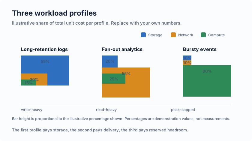
The examples share one lesson: the "expensive" meter is different in each case, so a single headline unit can only be right for one of them.
6Where Shared Storage changes the model
After working the model, a specific architectural condition becomes visible. If the dominant multipliers are replication hops and broker-local retained disks, the system is paying to move and store durability that the platform's own shared services already provide. The evaluation then shifts from "lower broker-hour cost" to a different question: can storage and compute be metered separately, with write durability no longer paid as replica movement between brokers?
Shared Storage architecture answers that question directly. It keeps Kafka semantics and the protocol surface while moving durable data to shared storage, so brokers shrink to stateless compute that can scale without moving the log data that gives them their identity. AutoMQ, a Kafka-compatible streaming platform, is one system built this way: it stays Kafka-compatible, writes incoming data through a WAL store, and persists the stream in S3-compatible object storage.
In the three-meter model, that changes which terms appear in each column. Storage becomes an object-storage line with object requests and WAL capacity on the side, instead of a count of provisioned broker disks. Network loses the broker-to-broker replica hops for durability in supported topologies because durability comes from the storage layer, although producer-to-broker, consumer, and cross-region paths still exist and still need accounting. The docs around eliminating inter-zone traffic show the conditions under which cross-AZ paths can be removed rather than just reduced. Compute becomes the broker count needed to serve traffic, decoupled from retained bytes, with stateless brokers and self-balancing doing the work that used to require data relocation.
This is not a claim that object storage makes everything free. It is a statement about which meter moves. The same normalization applies, the same three questions still require workload data, and a fair comparison still must include WAL capacity choice, object request and retrieval cost, and probe the deployment's actual topology before assuming any traffic term is zero.
7Where each architecture fits the comparison
Where does the model land? Run the three profiles from before through both columns.
- A long-retention logging team with consumers that stay on the tail will see the storage meter dominate; a Shared Storage architecture reduces that line by moving retained data to object storage and scaling brokers independently of it.
- A fan-out analytics team will still pay delivery hops, but the replication-fan-out interaction that inflated broker counts may shrink when replica traffic no longer exists and broker capacity follows consumers rather than retained partitions.
- A bursty events team spends its effort on compute; a design whose brokers are stateless is easier to scale down after the peak because shrinking does not require relocating log data.
The point of the table is not that one architecture wins. It is that each profile has a different target, and the architecture that wins is the one that reduces the specific multiplier that dominates the profile.
8Pick one byte and price it yourself
Take a real topic from your own cluster and put it through the model. Measure producer bytes per second, replication factor, retention window, consumer group count, and the zone placement of producers, brokers, and consumers. Convert each candidate's quote into the same denominator, keeping compression, replica, and access assumptions written down. Then ask, for each of the three meters, which architecture actually changes the number, and which one only moves the line between columns.
You will find that the useful question was never "what does Kafka cost?" It was "what does this byte cost, for how long, across how many hops, and at whose peak?"
If the exercise shows that replication traffic and broker-local retained disks are the lines moving your bill, test the same workload on a Shared Storage architecture before the next renewal. Start an AutoMQ evaluation with those measured inputs: producer rate, retention policy, consumer fan-out, and zone layout, rather than a headline throughput number.
9References
- Apache Kafka: Design
- Apache Kafka: Replication
- Apache Kafka: Topic Configuration
- Apache Kafka: Quotas
- KIP-405: Kafka Tiered Storage
- AutoMQ: S3Stream Shared Streaming Storage
10FAQ
10.1What does "cost per byte" actually mean for Kafka?
It means picking a denominator (produced, retained, or delivered bytes) and dividing by it the total monthly cost for storage, network, and compute. Until the denominator is defined, two cost-per-byte figures describe different work.
10.2Which Kafka cost dominates: storage, network, or compute?
It depends on the workload profile. Retention and replica-heavy topics are usually storage and replication traffic dominated; fan-out and replay-heavy topics are network dominated; spiky topics with idle capacity are compute dominated.
10.3How do I compare Kafka pricing when every vendor quotes different units?
Convert every unit to a single workload denominator you define. State whether the denominator is compressed or uncompressed, then convert broker-hours, partition fees, and quota units into that denominator using your own producer, retention, and consumer assumptions before comparing.