
Table of Contents
Table of Contents
The throughput graph doubles, but the Kafka bill grows faster than throughput. In the monthly review, the platform team points to broker hours, the network team points to data transfer, and finance sees a storage line that keeps rising after traffic has leveled off. Everyone can be looking at a real part of the bill.
The mistake is treating Kafka cost as one price for one unit of throughput. A cloud deployment pays for useful bytes and for work created around them: capacity reserved for peaks, copies moved between failure domains, data kept for retention, and reads that bring older data back into the path. A cost review must separate those curves, then decide whether configuration can change them or whether the storage architecture is creating the charge.
1Scale exposes the pricing model, not the other way around
Kafka gives a workload several ways to become larger without increasing producer ingress. A topic may keep data for a longer window. More consumer groups may read the same records. A replay job may fetch old segments while the normal tailing workload continues. A recovery event may move replicas or rebuild local storage. None of those changes has to show up in the producer's bytes-per-second metric.
The cloud sees the resulting resource use through different meters. Compute is often metered by instance or broker time. Block storage is metered by provisioned capacity and, depending on the service, performance characteristics. Object storage adds storage, request, and retrieval dimensions. Network charges depend on the path, region, availability-zone boundary, direction, and service-specific pricing rules. A managed Kafka price may bundle some of these meters, but bundling does not remove the underlying work.
That is why a useful cost model starts with paths instead of product names. Draw where a logical record is written, copied, retained, read, and exported. Assign each edge and resource to the account or team that pays for it. This shows which line should change when the workload changes.
2The three cost drivers and how they compound
2.1Broker headroom is a charge for the peak you may not use
Broker capacity covers more than average ingress. It also absorbs connections, partition leadership, request bursts, consumer fetches, metadata, cache pressure, and failure headroom. Teams commonly size for a peak, add room for uneven partitions, and then keep the fleet at that size because moving partitions during scale-in has a risk and an operational cost.
This is not an argument against headroom. A cluster full at the average rate has no room for a burst or a failed node. The FinOps question is whether reserved headroom protects a service objective or compensates for a storage model that makes capacity changes difficult. Compare utilization percentiles with the safe operating limit, and check whether one hot partition or broker sets fleet size.
2.2Replication turns logical writes into network work
In a traditional multi-AZ Kafka layout, replicas are maintained on different brokers and often in different availability zones. A producer sends one logical record, while the cluster may transmit additional copies to keep the configured replication factor in sync. The exact billable volume depends on the leader and follower placement, the provider's treatment of the path, compression, retries, reassignments, and whether traffic crosses a charged boundary.
Use a model rather than a slogan:
billable replication volume
= logical bytes written
  x replica traffic created by the topology
  x fraction that crosses a billable boundary
  x direction and provider billing rules
This formula is deliberately not a universal multiplier. A three-zone topology, a single-zone topology, and a workload with frequent reassignment produce different paths. The important control is to measure the path before applying the unit price. VPC flow records, provider billing dimensions, broker network metrics, and rack or zone assignments can be reconciled to do that.
2.3Storage cost follows retention and access, not only ingress
Retention keeps data after its first consumer has finished. Compaction rewrites selected records. Replays fetch historical segments. These behaviors determine how much storage is occupied and how often the system touches data that is not part of the current tail.
Local or block storage makes this relationship visible as broker capacity. A team may add disk to keep a long retention window, then add brokers when disk or recovery time becomes the limiting constraint. Tiered storage can move older bytes to object storage, but it does not automatically remove broker compute, replication, metadata, or read-request costs. Apache Kafka's topic settings and tiered-storage design documents are useful starting points, but the bill still depends on the actual access pattern.
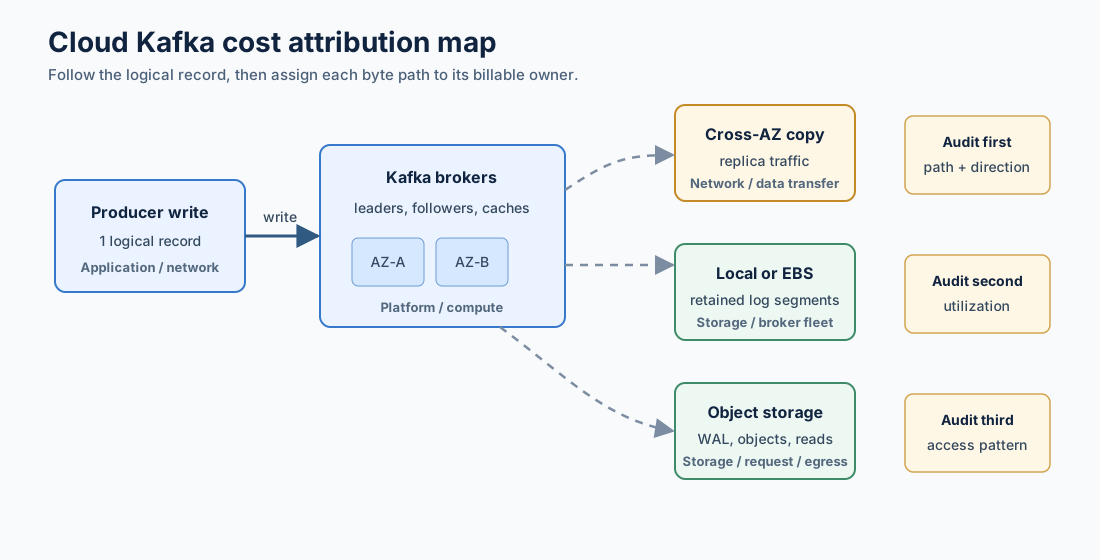
These drivers compound because one architectural choice can touch all three. Broker-local retained data makes scale-in a data movement exercise. A multi-AZ replication policy adds network work to the durable-write path. A longer retention window increases the amount of data that must be placed, recovered, and potentially reread. The bill does not say which dependency caused the increase, so the audit has to reconstruct it.
3Which line to audit first: a triage order
The first check should be the one most likely to explain why the bill changed. Use this order when throughput is not enough to explain the increase.
- Trace traffic direction. Start with data transfer, inter-AZ, inter-region, private endpoint, and egress dimensions. Separate producer-to-broker traffic, broker-to-broker replication, consumer fetches, replay reads, recovery movement, and exports. A network line that rose faster than ingress is a strong signal that topology or read behavior is involved.
- Check capacity utilization. Compare broker CPU, network, disk throughput, request rate, partition count, and storage utilization over the same billing window. Use percentiles and the busiest broker, not only a fleet average. If the fleet is lightly used except for a short peak, ask why scale-in is unsafe or slow.
- Inspect storage access. Map topic retention and compaction to stored bytes, then separate tailing reads from historical reads. Check whether a replay, backfill, or consumer outage created a read burst. Object storage may lower the price of retained bytes while request and retrieval activity becomes the larger variable.
- Only then compare unit prices. A lower price per GB will not fix a path that moves several GB for every logical GB, and a smaller broker will not fix a retention policy that keeps the same data elsewhere. Apply the provider's regional price to the verified quantity and record the assumptions.
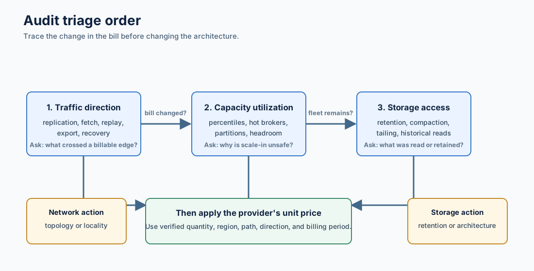
This order also prevents a common accounting error: assigning every data-transfer line to the application team. The team producing events may own logical ingress, while the platform team owns replication topology and the data owner controls retention. The invoice is shared evidence, not an ownership map.
4Four ways to lower the bill and where each breaks
Start with the changes that preserve the current architecture. They are often enough when the bill is caused by drift rather than by a structural coupling.
- Clean up retention and replay behavior. Remove abandoned topics, set retention with the data owner, review compaction, and give backfill jobs an explicit budget. This helps when retained bytes or cold reads dominate. It does not change the cost of keeping replicas across zones.
- Change placement and traffic locality. Review rack awareness, client routing, consumer placement, and cross-zone paths. Locality can reduce a particular network charge. It does not remove replication traffic when durable copies still live on separate brokers, and it can trade network cost for a narrower failure-domain choice.
- Right-size or schedule capacity. Use measured peak windows and partition balance to test scale-in. This can reduce broker-hours when utilization is low. It is a poor fit when the cluster cannot shrink without moving large local datasets, or when unpredictable recovery and burst requirements make scheduled scaling unsafe.
- Evaluate a shared-storage architecture. A Kafka-compatible system can separate broker compute from durable stream storage. If records are written to shared storage through a WAL and do not require broker-to-broker durable copies, the architecture can remove the specific cross-AZ replication path that was driving the bill. The trade-off moves to object-storage requests, read-back behavior, WAL media, cache sizing, and the deployment's own network boundaries.
The fourth path is not automatically the right answer. Test it when the worksheet keeps showing the same relationship: broker capacity is sized by retained data, scaling requires data movement, and cross-zone replication recurs. A neutral comparison should keep the same retention, producer rate, consumer fan-out, availability objective, and recovery test on both sides.
5How AutoMQ fits the evaluation
Once the audit shows that broker-local durability is the constraint, the required capability is specific: Kafka protocol and semantics for applications, durable storage that is not owned by one broker, and a scaling path that does not copy the retained dataset every time compute changes. That is the point where a platform such as AutoMQ belongs in the evaluation, not at the start of the cost discussion.
AutoMQ uses a Shared Storage architecture. Its brokers handle Kafka requests, partition leadership, scheduling, and caches, while S3Stream writes durable stream data through WAL storage and S3-compatible object storage. The S3Stream overview describes the storage layer; the relevant cost question is how that design changes the bytes in your own topology.
For a workload that currently pays to keep durable broker copies across zones, shared storage can remove the broker-to-broker replication path from the write design. Stateless brokers can also make replacement and capacity changes less dependent on moving partition data. Those are architectural effects, not a promise of a fixed percentage reduction. S3 request volume, catch-up reads, egress, WAL selection, caching, and the number and placement of brokers still need to be measured.
Deployment boundary matters as well. A BYOC design keeps the data plane and its storage choices in the customer's cloud environment, but it does not make provider pricing disappear. Validate object-storage access, IAM, private networking, recovery behavior, and any control-plane or marketplace charges against the account that will receive the bill. The AutoMQ environment documentation is a starting point for that boundary review.
6A worksheet you can reuse next quarter
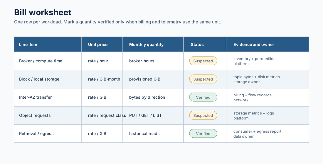
Use one row per workload or topic family. The row should describe the bytes and the path well enough that a finance partner can reproduce the calculation without knowing Kafka internals.
| Line item | Unit price | Monthly quantity | Suspected or verified | Evidence and owner |
|---|---|---|---|---|
| Broker or compute time | Provider rate / hour | Broker-hours by size | Suspected until utilization is joined | Instance inventory, utilization percentiles, platform |
| Block or local storage | Provider rate / GiB-month | Provisioned GiB and performance tier | Suspected until retention is mapped | Topic bytes, disk metrics, storage owner |
| Inter-AZ or inter-region transfer | Provider rate / GiB | Verified bytes by direction and path | Verify first when the line rose faster than ingress | Billing export, flow records, network |
| Object-storage requests | Provider rate / request class | PUT, GET, LIST, and lifecycle requests | Suspected until access pattern is separated | Storage metrics, request logs, platform |
| Object-storage retrieval or egress | Provider rate / GiB | Historical reads and external transfer | Verify for replay-heavy workloads | Consumer metrics, egress report, data owner |
Do not fill the table with one cluster-wide average. Record the region, availability zones, compression assumption, replication factor, retention window, average and peak ingress, consumer fan-out, and the billing period. Mark a quantity as suspected when it is inferred from a configuration value, and verified only when the billing or telemetry record measures the same unit.
The worksheet should produce an action, not a prettier invoice. For replication traffic, capture a representative topic's leader and follower paths and reconcile the result with the provider's data-transfer dimensions. For idle capacity, test a controlled scale-down window with a rollback condition. For storage access, run a normal tailing period and a representative replay separately. Re-run the table after the next material topology or retention change.
The decision is then easier to explain: keep the current Kafka shape and tune the line that evidence identifies, or test a different storage boundary because the current one makes compute, copies, and retained bytes rise together. Return to the bill that started the review. The useful question is no longer why Kafka is expensive in the abstract, but which bytes your architecture is asking the cloud to store, move, and read twice.
For a workload-specific comparison, bring the worksheet to an AutoMQ BYOC evaluation with the same traffic, retention, consumer, and recovery assumptions. A cost decision is stronger when both architectures have to explain the same bill.
7References
- Apache Kafka design documentation
- Apache Kafka replication documentation
- Apache Kafka topic configuration reference
- Apache Kafka KIP-405: Tiered Storage
- AWS EC2 On-Demand pricing and data transfer
- AWS EBS pricing
- AWS S3 pricing
- AutoMQ architecture overview
8FAQ
8.1Why can a Kafka bill grow faster than producer throughput?
Producer throughput measures logical ingress, not every resource action. Replication, consumer fan-out, replay, retention, recovery movement, broker headroom, and storage requests can grow independently. Trace the bytes and resource hours before comparing the bill with ingress.
8.2Should I reduce Kafka replication factor to lower cost?
Replication factor is part of the durability and failure-domain design. Model the failure objective, recovery window, and availability requirement first. A lower factor may change a network line while creating a recovery risk that the cost model does not capture.
8.3Is tiered storage enough to solve cloud Kafka cost?
It can help when retained bytes on local or block storage are the main driver, especially when historical reads are infrequent. It does not automatically remove broker compute, replication traffic, metadata work, or object-storage request and retrieval charges. Test the access pattern that produced your bill.
8.4When should I consider shared storage?
Consider it when routine retention, placement, and capacity changes have been checked and the recurring cost still comes from coupling broker count to retained data and cross-zone replication. Compare the same workload and recovery objective, then include object-storage and network costs in the result.