
Table of Contents
Table of Contents
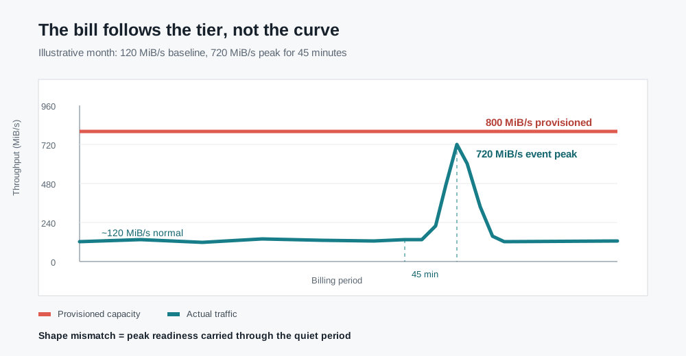
At 09:00 on the first day of a seasonal promotion, an Apache Kafka platform team has to choose between two uncomfortable numbers. The normal workload is about 120 MiB/s, but a similar event reached 720 MiB/s for 45 minutes. The budget spreadsheet therefore reserves an 800 MiB/s throughput tier for the whole billing period. The team accepts the idle capacity because a throttle during the event would be harder to explain than a large fixed line item.
That is a rational decision when the event is frequent, the peak is difficult to predict, or the service-level objective requires capacity to be ready immediately. It becomes expensive when the 720 MiB/s peak is the exception and the cluster spends most of its time near 120 MiB/s. The same provisioned-throughput model that makes the budget legible can then charge for a traffic shape the workload no longer has.
The useful question is not whether provisioned throughput is good or bad. It is whether the purchased capacity curve matches the observed curve, including the height, duration, ramp, and time available to scale. That distinction matters for Kafka provisioned throughput, MSK provisioned throughput cost, and any service that packages capacity into tiers.
1Predictability is a product, with a price
Provisioned throughput sells certainty before it sells bytes. A provider exposes a capacity boundary, a tier, or a configured throughput allowance, and the buyer pays for that reservation according to the service's current pricing rules. The exact meter varies by provider, region, broker type, storage mode, and feature selection. For an AWS workload, check the live Amazon MSK pricing page and the provisioned-cluster documentation rather than copying a rate into a long-lived model.
The trade is easy to understand. A team that provisions 800 MiB/s can plan around 800 MiB/s without asking whether an autoscaler will react before producers time out. It has a clear ceiling for capacity reviews, and it can align the allowance with a response-time objective. For steady traffic, that certainty can be worth carrying some unused headroom.
The price of certainty appears when the workload's shape changes. A tier sized for a launch window may stay in place after the launch. A replay job may use a high read rate for an hour and then disappear. An event-driven workload may move from a quiet baseline to a sharp peak faster than capacity can be changed. In each case, the provider is not necessarily overcharging. The customer is paying for readiness, while using only part of it.
Throughput is not the whole Kafka cost model. Replication, consumer fan-out, retention, storage, cross-zone paths, partition count, request rate, and monitoring may be billed or resourced separately. Keep those dimensions separate instead of treating a throughput unit as the price of a complete cluster.
2When your curve changes shape, the math breaks
Return to the illustrative promotion. Suppose the workload averages 145 MiB/s over the month, reaches 720 MiB/s at the event, and uses an 800 MiB/s provisioned tier. The peak-to-average ratio is about 5.0, while average utilization of the purchased tier is about 18%. Neither number proves that the tier is wrong. Together, they show why a monthly average can hide a large readiness payment.
The arithmetic should remain explicit:
Provisioned model: provisioned capacity x billed time x provider rate
Usage-shaped model: metered bytes or capacity used x provider rate
Shape mismatch: purchased peak - normal demand, carried outside the burst window
These are model shapes, not interchangeable provider invoices. The first line may be charged by storage throughput, broker capacity, or another service-specific unit. The second may include minimums, request charges, network, or separate compute. Use the formula to expose assumptions, then fill in current rates from the provider's pricing page.
The mismatch has two forms:
- Peak overbuying: a short event forces the entire service onto a higher tier, even if the tier cannot be released quickly after the event.
- Low-period underuse: the purchased capacity remains available during nights, weekends, or inactive seasons, but the bill does not fall with utilization.
There is a failure mode on the other side. A lower tier may depend on throttling, retries, or delayed capacity changes, moving the cost into producer latency, consumer lag, or a missed processing window. Quotas can contain one workload, while retention, compaction, replication, and min.insync.replicas address different objectives. None makes an undersized tier safe by itself.
3Peak-to-average ratio: the number that tells you
Peak-to-average ratio is useful because it describes the shape rather than the total volume. Calculate it for a defined window:
peak-to-average ratio = peak rate in the window / average rate in the window
Use the same unit and signal on both sides. Inspect producer bytes, consumer bytes, and request or partition pressure separately. Steady ingest can hide a bursty replay consumer, while stable bytes can hide a request-rate spike.
Duration gives the ratio meaning. A 5.0x peak lasting 45 minutes asks a different question from a 5.0x peak lasting two days. Record time above threshold, ramp-up, ramp-down, and the full capacity-change time, including provider limits, startup, partition movement, cache warm-up, and client recovery. If the burst finishes first, an elastic price may not remove the standing buffer.
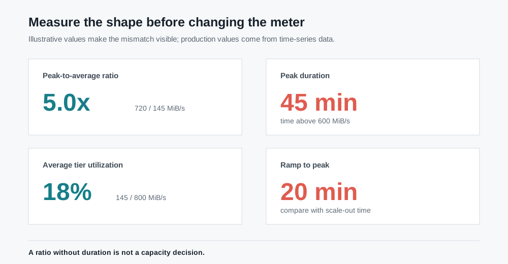
The following worksheet is enough to make the first decision:
| Metric | Illustrative observation | Question it answers |
|---|---|---|
| Normal rate | 120 MiB/s | What capacity is used most of the time? |
| Monthly average | 145 MiB/s | How much does the long window hide? |
| Event peak | 720 MiB/s | What capacity must be ready? |
| Peak-to-average | 5.0x | How far is the shape from the mean? |
| Time above 600 MiB/s | 45 minutes per event | Can the peak be scheduled or isolated? |
| Ramp to peak | 20 minutes | Can capacity change before clients feel it? |
| Scale-in time | Measure in the pilot | How long does the extra cost persist? |
The figures above are illustrative assumptions, not a benchmark or a pricing quote. Replace them with time-series data from the producer, consumer, broker, and billing systems. The important output is not a single ratio. It is a relationship between peak height, peak duration, and the time required to release capacity.
4Three pricing paths and the shapes they love
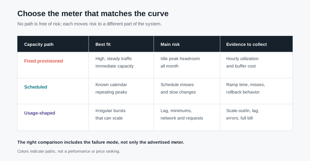
Once the curve is visible, compare pricing paths against the workload's failure mode. A simple matrix keeps the discussion neutral:
| Capacity path | Fits best | Main cost risk | Test before choosing |
|---|---|---|---|
| Fixed provisioned tier | High and steady traffic, strict immediate-capacity objectives | Paying for the peak during every quiet period | Utilization by hour and the cost of the standing buffer |
| Scheduled capacity | Repeating daily, weekly, or seasonal peaks | An unplanned event arrives outside the schedule | Schedule miss rate, change lead time, and rollback behavior |
| Usage-shaped or elastic capacity | Irregular bursts where capacity can follow demand | Scale-out lag, minimum charges, quotas, or request and network fees | Time to capacity, time to scale in, lag, errors, and total bill |
Fixed capacity can be the least risky choice when a workload runs near its ceiling, has a strict latency objective, or cannot tolerate scale-out delay. The test is whether idle capacity is a deliberate reliability margin or a historical peak nobody revalidated.
Scheduling works when the calendar predicts demand. It is weaker when an external signal triggers the event, the ramp is faster than the schedule change, or a failed scale-in leaves the larger shape in place.
Usage-shaped services can reduce the penalty for an empty night, but a usage meter does not make every cost variable. Check minimums, request rates, storage growth, egress, cross-zone traffic, retention, warm compute, read fan-out, and replay. Compare the full workload boundary, not only the number beside "throughput."
The third path can be architectural. If durable data is coupled to broker-local disks, adding or removing serving capacity may require data movement. Ask which state must move when the curve changes.
5What elastic storage and compute need to prove
The capacity model is only as flexible as the slowest state transition behind it. Before selecting an architecture for bursty Kafka traffic, require evidence for five properties:
- Protocol continuity: Kafka clients and tools can be tested without rewriting the application contract.
- Separate durable state: serving nodes can change without copying the retained dataset for every capacity event.
- A bounded write path: WAL (Write-Ahead Log) or equivalent storage has visible failure, recovery, and durability boundaries.
- Partition-aware placement: hot-partition movement, leader changes, and cache warm-up remain observable.
- A complete cost meter: object requests, retained bytes, compute, network, and operations are included.
This is where a Shared Storage architecture becomes relevant. AutoMQ keeps the Kafka protocol and semantics while using shared storage in which brokers serve compute and routing roles, and S3Stream writes durable stream data through WAL and object storage. In that model, a scaling policy can follow actual partition traffic instead of selecting a permanent throughput tier in advance. The architectural property matters because a broker capacity change does not have to mean moving every retained partition replica with the broker.
That property is not a promise of a particular speed or cost. WAL type, object storage, cache state, partition distribution, retention, region, and control-plane policies affect the result. AutoMQ BYOC also leaves cloud resources, network placement, and provider charges inside the customer's environment.
For teams evaluating it, the Kafka compatibility documentation defines the application boundary. The shared storage overview and WAL storage documentation define the storage path to test. Ask whether that separation removes the state movement keeping the capacity curve flat.
6A pilot for leaving the tiered comfort zone
Do not begin with the largest production cluster. Start with representative topics and a repeatable shape. Preserve message size, partition distribution, retention, consumer fan-out, acknowledgment settings, and failure-zone placement so the cost change remains explainable.
Run four windows:
- Baseline: hold the normal rate long enough to observe steady compute, storage, cache, and network behavior.
- Planned burst: ramp toward the expected event peak with a known start time.
- Unplanned burst: introduce a faster ramp or a replay pattern that the schedule did not predict.
- Scale-in: return to baseline and keep observing until capacity, cost, lag, and cache behavior settle.
Capture the same measures in every window:
| Area | Measures to retain |
|---|---|
| Service | Produce and fetch latency, errors, throttles, consumer lag |
| Shape | Peak-to-average ratio, duration, ramp, and scale-in time |
| State | Partition ownership, leader movement, cache hit behavior, WAL pressure |
| Cost | Compute, provisioned or usage throughput, object requests, retained bytes, network |
| Recovery | Broker loss, storage interruption, replay time, and client reconnect behavior |
Use the current provisioned tier as the control and compare equal workload windows. A usage-shaped option should show the peak cost, storage-access cost, and operational work as well as a lower quiet-period line. If scale-in does not happen, the model is not elastic for this workload.
The decision can stay concrete. Keep fixed provisioned capacity when the workload is high and steady, the peak is safety-critical, or scale-out time is longer than the burst. Schedule capacity when the calendar is trustworthy and the provider can change capacity before the event. Test a Shared Storage architecture with elastic compute when retained data and broker capacity are coupled, and verify object storage, WAL, network, and recovery costs under the real traffic shape.
The 800 MiB/s tier in the opening example may still be correct. The difference is that the team now knows whether it is buying an active requirement, a short-lived event, or a historical peak that survived because nobody measured scale-in. That is the useful meaning of predictable pricing: not a fixed number, but a number whose assumptions remain visible.
7References
- Amazon MSK pricing
- Amazon MSK provisioned clusters
- Apache Kafka design and replication
- Apache Kafka topic configurations for retention and compaction
- Apache Kafka quotas and throttling
- AutoMQ architecture overview
- AutoMQ continuous self-balancing
8FAQ
8.1Is provisioned Kafka throughput a bad pricing model?
No. It is a reasonable fit for high, steady traffic or a service that must have capacity ready before demand arrives. The mismatch appears when an irregular peak determines the tier and the platform cannot release that capacity during the long quiet period.
8.2What is peak-to-average ratio in Kafka capacity planning?
It is the peak rate divided by the average rate for the same signal and time window. Calculate it separately for producer bytes, consumer bytes, and request or partition pressure. Always pair the ratio with peak duration and ramp time.
8.3How should I model MSK provisioned throughput cost?
Start with the current AWS pricing page and identify the broker type, region, storage mode, provisioned-throughput option, retention, network path, and monitoring features. Then map hourly capacity, storage, data transfer, and request behavior to your measured workload. Do not treat an illustrative throughput tier as a quoted price.
8.4Can AutoMQ remove the need for throughput tiers?
AutoMQ's Shared Storage architecture and stateless brokers can reduce the data-movement constraint behind broker capacity changes, but they do not remove workload limits or cloud-resource charges. Test scaling time, partition placement, WAL, cache warm-up, object-storage access, retention, network, and scale-in behavior under your own traffic curve.
8.5What should a Kafka burst-pricing pilot prove?
It should prove both directions: capacity reaches the burst without unacceptable lag or errors, and the system returns toward baseline after the burst. Include planned and unplanned ramps, the full cost meter, and a failure or recovery window. A test that only demonstrates scale-out does not validate the budget model.
When the next event planning meeting asks for another permanent tier, bring the curve first. You may still buy the tier, but you will know whether it is paying for service protection, an architectural constraint, or a peak that no longer exists. To test the Shared Storage path with your own Kafka workload, start an AutoMQ evaluation.