
Table of Contents
Table of Contents
A platform team is asked to create a topic for an event stream that peaks at 480 MB/s. Someone reaches for the partition count from another cluster, rounds it up, and moves on. The topic works in a load test. A month later, the bill includes more broker memory and storage than expected, consumers still fall behind during recovery, and nobody can explain which assumption produced the number.
That failure is common because partition count is asked to do several jobs at once. This is the Kafka partition sizing problem in practice: the count provides write and read parallelism, creates units for consumer assignment, affects broker metadata and file state, and interacts with replica placement and retained bytes. A count that is generous for one constraint can be wasteful for another.
The defensible answer is the smallest tested count that satisfies throughput, latency, recovery, ordering, and operating-cost constraints together. The worksheet makes each input visible, keeps units attached to the calculation, and separates a Kafka limit from a limit imposed by a particular broker shape or cloud bill.
1More partitions is a reflex, not a plan
More partitions can increase parallel work, but they do not create throughput by themselves. A producer still has to distribute records across keys, a broker still has to serve requests, and a consumer group still has to process the assigned partitions. If one key receives most of the traffic, adding partitions will not move that key's records to several partitions while preserving order.
Fewer partitions have a different failure mode. A consumer group may have idle consumers because one active consumer owns too much work, or a hot partition may accumulate lag while other partitions are quiet. The choice is therefore not "many versus few." It is a capacity decision with an application constraint attached.
Start by writing down the boundaries that cannot be averaged away:
- Ordering boundary: records with the same key stay in one partition when per-key order matters. A partition increase can change the mapping for future records, so treat it as a data and consumer-behavior change, not only a capacity knob.
- Parallelism boundary: one consumer in a group can own at most one partition at a time. A group that needs 48 active workers needs at least 48 useful partitions, although it may need more to absorb skew and uneven processing time.
- Recovery boundary: a topic that is acceptable at steady state may fail its recovery objective if the consumer group cannot drain backlog quickly enough after an outage or planned pause.
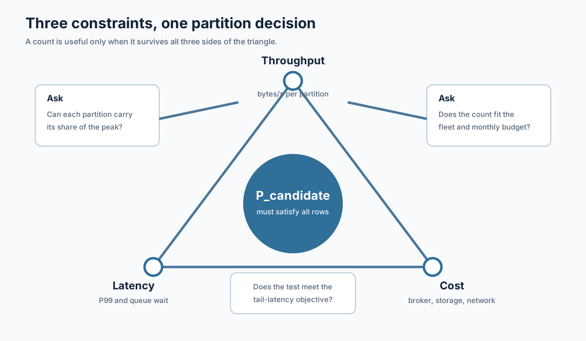
An inherited rule such as "use 100 partitions for a busy topic" hides the workload shape and makes spare capacity impossible to review. The three-way view below is a better starting point.
2Three constraints: throughput, latency, cost
Partition sizing starts with a rate, but the rate needs context. Use record rate when sizes are stable, byte rate when payloads vary, peak rate for a peak service objective, and monthly average only for storage or spend estimates. Throughput asks whether a partition can carry its share without queue growth. Latency asks whether it can do so within the percentile target. Cost includes the metadata, connections, monitoring, local storage, and replica movement that partition count can multiply.
Keep the constraints separate until the end. A worksheet should contain at least these rows:
| Constraint | Input with units | What a failed row looks like |
|---|---|---|
| Producer throughput | Peak bytes/second, records/second, and measured safe bytes/second/partition | Producer throttling or growing broker queues |
| Consumer throughput | Peak bytes/second per group and measured safe bytes/second/partition | Consumer lag or a recovery window that is missed |
| Tail latency | P95/P99 target in milliseconds and load-test result at the candidate count | Queue wait or fetch latency rises at the peak |
| Parallelism | Active consumers per group and processing time per record | Workers are idle while one partition stays hot |
| Recovery | Backlog bytes, drain window in seconds, and recovery bytes/second/partition | Backlog lasts longer than the service objective |
| Cost and limits | Broker-hours, retained bytes, replication factor, file handles, memory, and provider rates | The count fits traffic but not the fleet or budget |
Kafka replication factor is a durability and availability setting, while min.insync.replicas is an acknowledgment safety condition. Neither is a universal cost multiplier: check the write path, replica placement, storage model, provider, region, and billing path.
3The formulas, with units that survive review
Use measured safe capacity rather than a folklore number. Let B_peak be peak bytes/second, and let b_safe be the safe measured bytes/second for one partition under a stated test configuration.
P_write = ceil(B_peak / b_safe)
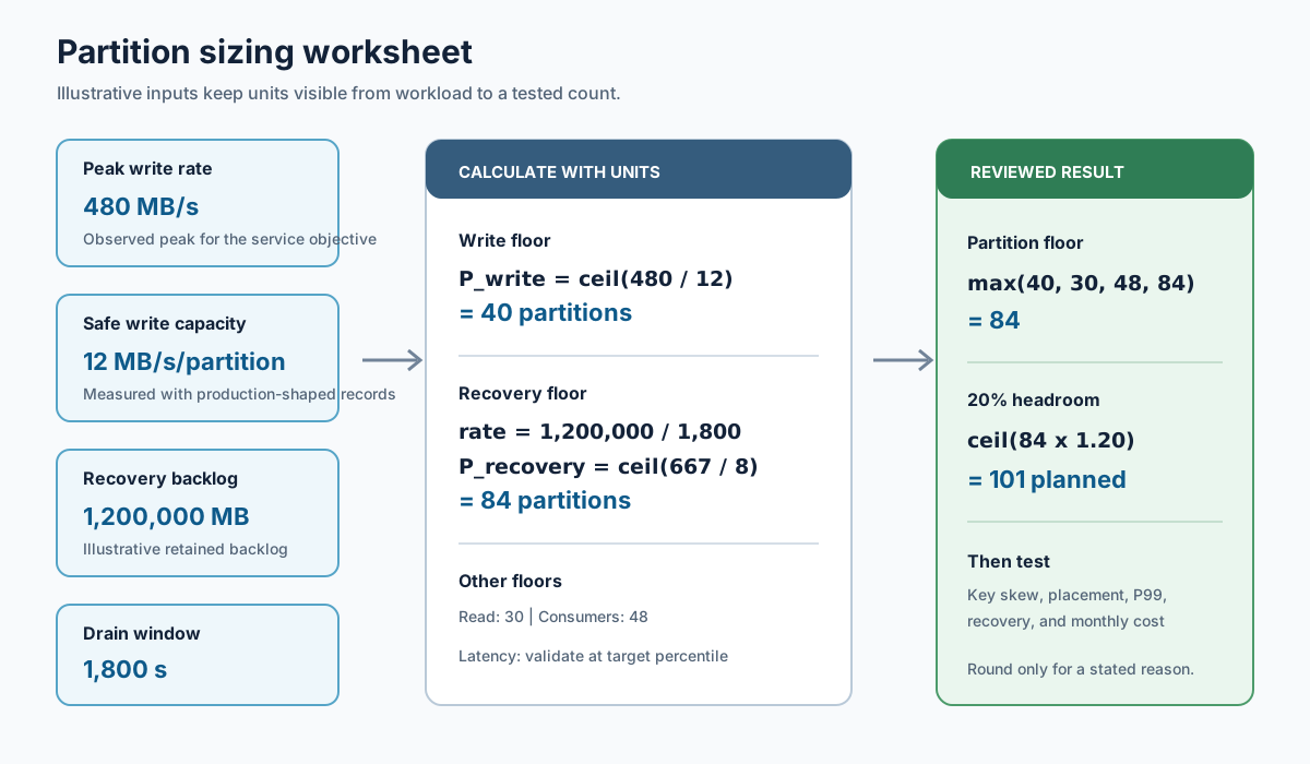
For example, if an illustrative test uses B_peak = 480 MB/s and measures b_safe = 12 MB/s/partition, then P_write = ceil(480 / 12) = 40 partitions. The result is not a Kafka constant. It is valid only for the record size, compression, acknowledgment mode, producer batching, key distribution, broker type, and latency target used in that test.
Run the same calculation for each important consumer group:
P_read(group) = ceil(B_read(group) / b_read_safe(group))
P_consumer(group) = active consumers required by the group
P_consumer is a floor for useful parallelism, not proof that the group will meet its latency target. A group with 48 workers may still need more than 48 partitions if record processing varies substantially or if one key dominates. Conversely, creating 500 partitions for 48 workers does not make the processing code 10 times faster.
For the illustrative worksheet, suppose one consumer group peaks at 300 MB/s and measures 10 MB/s/partition, giving P_read = ceil(300 / 10) = 30. The example also assumes 48 active workers.
Recovery deserves its own row. If L is backlog bytes, T is the allowed drain time in seconds, and b_recover_safe is the safe recovery rate per partition, then:
P_recovery = ceil((L / T) / b_recover_safe)
With illustrative assumptions of L = 1,200,000 MB, T = 1,800 seconds, and b_recover_safe = 8 MB/s/partition, the required recovery rate is 667 MB/s, so P_recovery = ceil(667 / 8) = 84 partitions. This can be larger than the steady-state write result. That is the point of keeping recovery visible.
The latency row is validated rather than invented from a universal formula. Treat it as a budget: T_budget = T_end_to_end - T_network - T_processing - T_storage. Test the candidate count at target load and record queue wait, produce latency, fetch latency, and consumer processing time at the selected percentile. If the byte-rate target passes but P99 does not, check batch size, key skew, broker saturation, and consumer code before adding partitions.
Now combine the floors:
P_floor = max(P_write, P_read(group 1..n), P_consumer(group 1..n), P_recovery)
P_planned = ceil(P_floor * headroom)
For the illustrative inputs above, P_floor = max(40, 30, 48, 84) = 84. A 20% planning margin gives ceil(84 * 1.20) = 101 partitions. A team may choose a nearby number that distributes cleanly across the tested broker count, such as 108, but that rounding is an operational choice that needs a placement and skew test. It is not evidence that 108 is inherently safer than 101.
Cost belongs beside the count, not after it. A generic monthly estimate can be written as:
monthly cost = broker-hours * broker rate
             + retained GiB * storage rate
             + network GiB * network rate
             + object requests * request rate
             + operations and observability cost
For broker-local storage, retained bytes are affected by ingest rate, retention seconds, replication factor, cleanup policy, and storage overhead. A first-order capacity row is B_ingest * retention_seconds * replication_factor, with units converted to GiB before applying a provider rate. Compaction, segment overhead, and free-space policy need separate allowances. For a shared-storage design, durable bytes may move to object storage while a WAL and cache remain broker-local. That changes which term dominates; it does not make the other terms zero.
Measure the partition tax too. Depending on the implementation, each partition can add log segments and file descriptors, metadata, request queues, monitoring series, cache entries, and replica-placement work. Put measured resident memory and file handles per partition into the worksheet:
broker partition load = total partitions assigned to broker
broker memory overhead = broker partition load * measured bytes/partition
Do not label a provider's maximum partition count as a capacity target. It is a boundary for a particular service configuration. An operating target comes from a test that includes broker count, replica factor, topic mix, consumer groups, connections, and failure or reassignment behavior.
4Using the worksheet without boiling the ocean
Apply the worksheet to one representative topic family first. The goal is to expose the assumption that makes the fleet expensive or the recovery objective fragile.
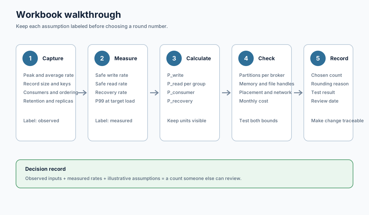
- Capture the workload. Record peak and average byte rate, peak record rate, average and maximum record size, compression, key cardinality, ordering requirements, producer count, consumer groups, retention, and replication settings. Mark every number as observed, measured, or illustrative.
- Measure safe per-partition rates. Use a production-shaped test. Keep the acknowledgment mode, batch settings, consumer processing, broker shape, and percentile target visible. Measure both steady state and a catch-up run.
- Calculate independent floors. Fill
P_write, everyP_read,P_consumer, andP_recovery. Add a latency test result beside the formulas. If a row has no unit, it is not ready for review. - Apply placement and budget checks. Test the candidate against partitions per broker, memory, file handles, connections, replica placement, retained GiB, network paths, and monthly cost. Recalculate for the smallest and largest plausible traffic shape.
- Choose, test, and record. Pick a count that has a reason for its rounding. Validate key skew, consumer assignment, restart behavior, recovery time, and operational tooling. Store the assumptions with the topic or platform decision so the next increase has a baseline.
Several scenarios change which row wins:
| Scenario | Row likely to dominate | Practical response |
|---|---|---|
| Large, evenly distributed event stream | Producer or consumer bytes/second | Measure safe per-partition rates and test tail latency at the peak |
| Many consumers with modest traffic | Consumer parallelism | Meet the active-worker floor, then check whether extra partitions add measurable value |
| One or a few hot keys | Key distribution and ordering | Fix the key strategy or isolate the hot workload; do not expect partition count alone to split an ordered key |
| Large restart backlog | Recovery bytes/second | Size for the drain window and test catch-up, not only normal traffic |
| Rapidly changing topic inventory | Broker metadata and operations | Include partition overhead and monitoring cardinality in the budget |
5What changes when partitions stop being tied to disks
In a broker-local Kafka layout, a partition is both a logical stream and a unit of local storage ownership. Its replicas occupy broker disks, retained bytes consume provisioned capacity, and reassignment can require moving a large amount of data between brokers. That coupling makes partition growth look like a storage-layout decision even when the original reason was consumer parallelism.
A Shared Storage architecture separates those concerns. Durable stream data can live in shared object storage while brokers retain the request-serving state, caches, metadata, and a write-ahead log or other recovery buffer required by the implementation. Increasing partitions can still increase metadata, file handles, connections, cache pressure, and scheduling work, but it does not automatically require the same proportional local-disk footprint or a full copy of every retained byte during a broker move.
That is the specific architectural capability to evaluate, not a blanket promise that partitions become free. AutoMQ is a Kafka-compatible streaming platform that uses Shared Storage architecture, WAL, caching, and object-storage access paths to change this partition-to-local-disk relationship. Its Kafka compatibility documentation is the right reference for client and protocol assumptions; its architecture overview describes the storage path.
AutoMQ's Self-Balancing can help redistribute serving ownership as partition traffic changes, while WAL and caching address the low-latency and recovery portions of the path. The limits still need a test: controller and broker metadata, open files, connections, request rate, cache working set, consumer parallelism, and object-storage access patterns. In AutoMQ BYOC, the customer still owns the cloud-region, provider pricing, permissions, network, and chosen WAL boundaries. Shared Storage architecture can loosen the partition-to-disk coupling; it does not erase a provider bill or a broker limit.
Hold client behavior and partition count constant. Measure broker scale-out, ownership movement, restart recovery, local storage, object-storage requests, cross-AZ paths, and total cost. This separates storage coupling from consumer code, key skew, or an undersized broker.
Return to the 480 MB/s example. If its 101-partition worksheet result is affordable and passes the recovery and P99 tests, changing platforms is unnecessary for partition sizing alone. If the count is correct for application parallelism but forces a local-storage layout and movement plan the team cannot operate, a shared-storage evaluation is justified.
6References
- Apache Kafka topic and partition documentation
- Apache Kafka replication and in-sync replica semantics
- Apache Kafka topic configuration reference
- Apache Kafka consumer configuration reference
- AutoMQ shared streaming storage architecture
- AutoMQ WAL storage
- AutoMQ continuous Self-Balancing
- AutoMQ inter-zone traffic architecture
7FAQ
7.1How many Kafka partitions should a topic have?
Use the maximum of the independently calculated write, read, consumer-parallelism, recovery, ordering, and platform-limit floors, then add a tested margin. There is no universal partition count. A number is defensible only when its workload, units, and test conditions are recorded.
7.2Does adding partitions always increase Kafka throughput?
No. It helps when partition-level parallelism is the bottleneck and keys distribute across partitions. It will not fix a hot key, slow consumer code, broker saturation unrelated to partition concurrency, or an unsuitable batch and acknowledgment configuration.
7.3How does replication affect partition cost?
Replication increases the amount of persisted or transferred data according to the configured replica placement and storage model. The exact cost depends on retention, cleanup policy, fault domains, network paths, provider rates, and whether storage is local, shared, or tiered. Treat replication factor and min.insync.replicas as separate worksheet inputs.
7.4Does shared storage remove Kafka partition limits?
No. It can reduce the coupling between partition count and broker-local durable storage or data movement. Broker metadata, connections, file handles, request handling, caches, consumer parallelism, recovery behavior, and object-storage access still need capacity tests.
Use the same worksheet and run a workload-specific AutoMQ evaluation, including the hot-key distribution and recovery window that produced the original decision.